Create a forest plot for simple data

forester(
  data,
  display_cols = c("Variable", "HR", "lower_95", "upper_95"),
  estimate_precision = 2,
  null_line_at = 1,
  font_family = "mono",
  x_scale_linear = TRUE,
  xlim = NULL,
  xbreaks = NULL,
  point_sizes = 3,
  point_shape = 16,
  label_hjust = 0,
  label_vjust = -1,
  label_color = "blue",
  label_size = 3
)

Arguments

data: Data frame (required). The information to be displayed as the forest plot.
display_cols: 4 columns stand for axis text and the forest data, default using c("term", "HR", "conf.low", "conf.high").
estimate_precision: Integer. The number of decimal places on the estimate (default 2).
null_line_at: Numeric. Default 0. Change to 1 if using relative measures such as OR, RR.
font_family: String. The font to use for the ggplot. Default "mono".
x_scale_linear: Logical. Default TRUE, change to FALSE for log scale
xlim: Vector. Manually specify limits for the x axis as a vector length 2, i.e. c(low, high)
xbreaks: Vector. X axis breaks to label. Specify limits in xlim if using this option.
point_sizes: Vector. Length should be equal to 1 or nrow(left_side_data). The sizes of the points in the center plot, where 3.25 is the default.
point_shape: Vector. Length should be equal to 1 or nrow(left_side_data). The shapes of the points in the center plot, where 16 (a filled circle) is the default.
label_hjust, label_vjust, label_color, label_size: hjust, vjust color and size for the label text.

Value

a ggplot object.

Examples

library(survival)

t1 <- ezcox(lung, covariates = c(
  "age", "sex",
  "ph.karno", "pat.karno"
))
#> => Processing variable age
#> ==> Building Surv object...
#> ==> Building Cox model...
#> ==> Done.
#> => Processing variable sex
#> ==> Building Surv object...
#> ==> Building Cox model...
#> ==> Done.
#> => Processing variable ph.karno
#> ==> Building Surv object...
#> ==> Building Cox model...
#> ==> Done.
#> => Processing variable pat.karno
#> ==> Building Surv object...
#> ==> Building Cox model...
#> ==> Done.
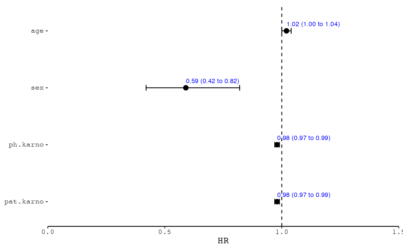
p <- forester(t1, xlim = c(0, 1.5))
p

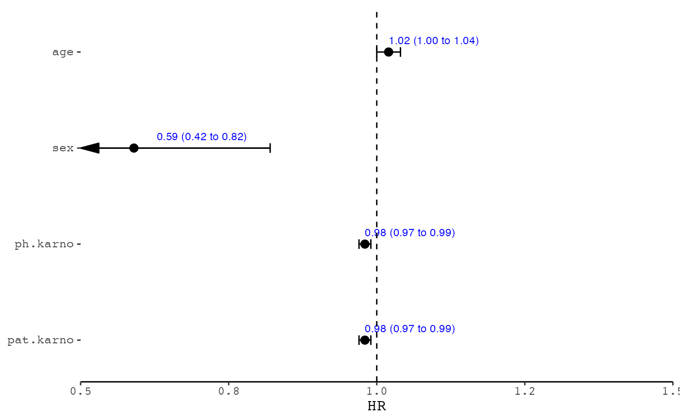
p2 <- forester(t1, xlim = c(0.5, 1.5))
p2