R基本绘图:创建与添加图形
王诗翔 · 2019-06-21
R 遵循画家模式。
高级绘图函数 + 低级绘图函数才能让图形丰富多样起来。
基本的低级绘图函数
| <U+51FD><U+6570> | <U+63CF><U+8FF0> |
|---|---|
| points() | <U+6570><U+636E><U+7B26><U+53F7> |
| lines() | <U+7EBF><U+6761> |
| segments() | <U+7EBF><U+6BB5> |
| arrows() | <U+7BAD><U+5934> |
| xspline() | <U+5149><U+6ED1><U+66F2><U+7EBF> |
| rect() | <U+77E9><U+5F62> |
| polygon() | <U+591A><U+8FB9><U+5F62> |
| polypath() | <U+591A><U+8FB9><U+5F62><U+8DEF><U+5F84> |
| rasterImage() | <U+4F4D><U+56FE><U+FF08><U+5728><U+56FE><U+5F62><U+4E0A><U+53EF><U+4EE5><U+6DFB><U+52A0><U+5916><U+90E8><U+56FE><U+7247><U+FF09> |
| text() | <U+6587><U+672C> |
添加图形
还是要一顿操作猛如虎,才能学到本事。
x = 1:10
y = matrix(sort(rnorm(30)), ncol=3)
plot(x, y[, 1], ylim = range(y), ann=F, axes = F, type="l", col="gray")
box(col="gray")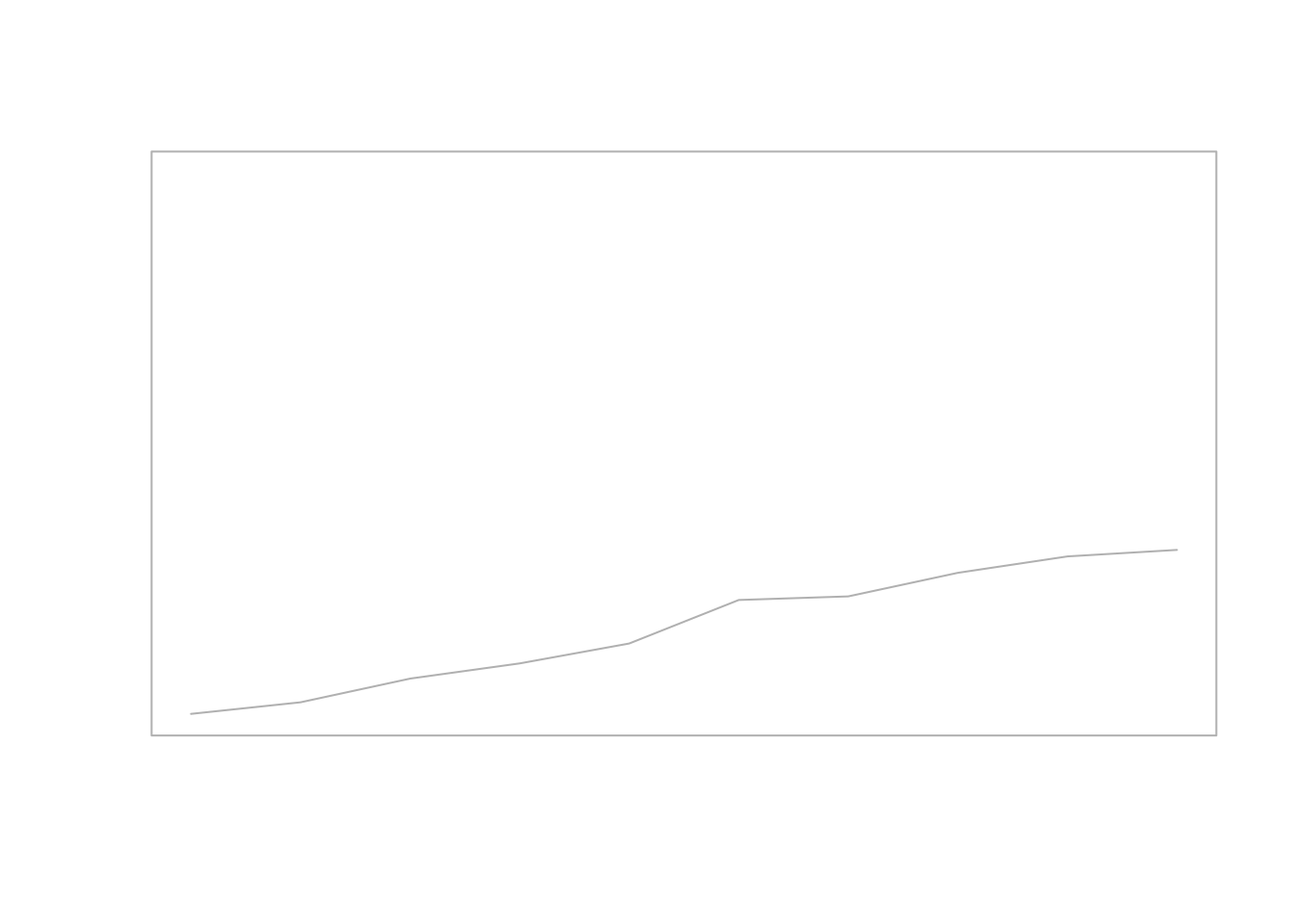
开始加东西。
plot(x, y[, 1], ylim = range(y), ann=F, axes = F, type="l", col="gray")
box(col="gray")

points(x, y[,1])
lines(x, y[,2], col="gray")
points(x, y[,2], pch=2)
lines(x, y[,3], col="gray")
points(x, y[,3], pch=3)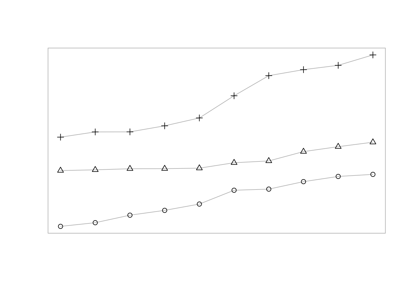
在点旁边添加文本有时候很有用,使用 pos 可以设置数据符号与文本之间的偏移量。
y = x = 1:5
plot(x, y, ann=F, axes=F, col="gray", pch=16)
box(col="gray")

text(x[-3], y[-3], c("right", "top", "bottom", "left"),
     pos=c(4, 3, 2, 1))
text(3, 3, "overlay")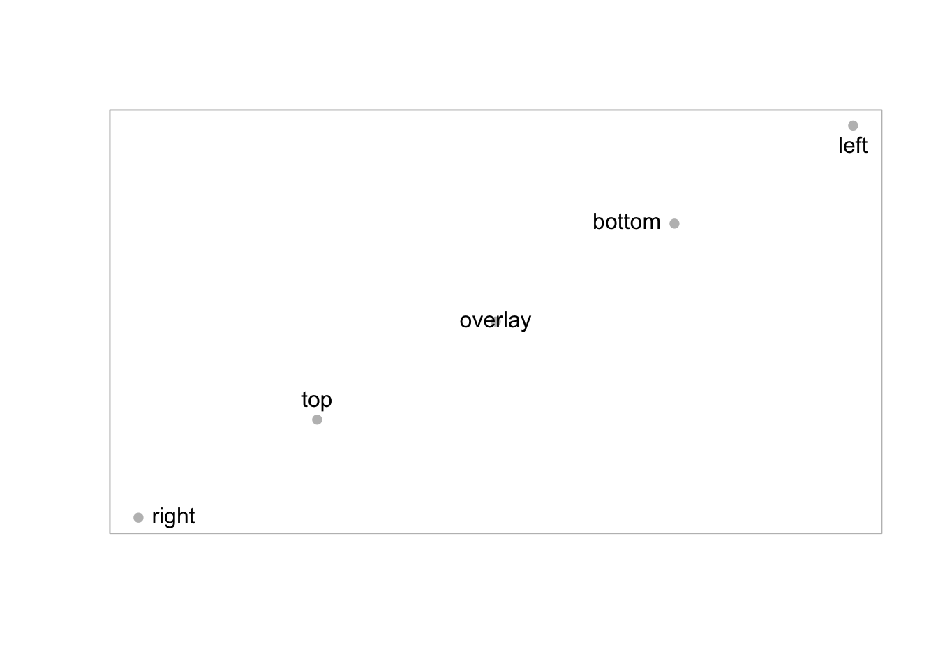
text() 还可以接受 R 表达式。
y = x = 1:5
plot(x, y, ann=F, axes=F, col="gray", pch=16)
box(col="gray")

text(x[-3], y[-3], c("right", "top", "bottom", "left"),
     pos=c(4, 3, 2, 1))
text(3, 3, ~ x^2)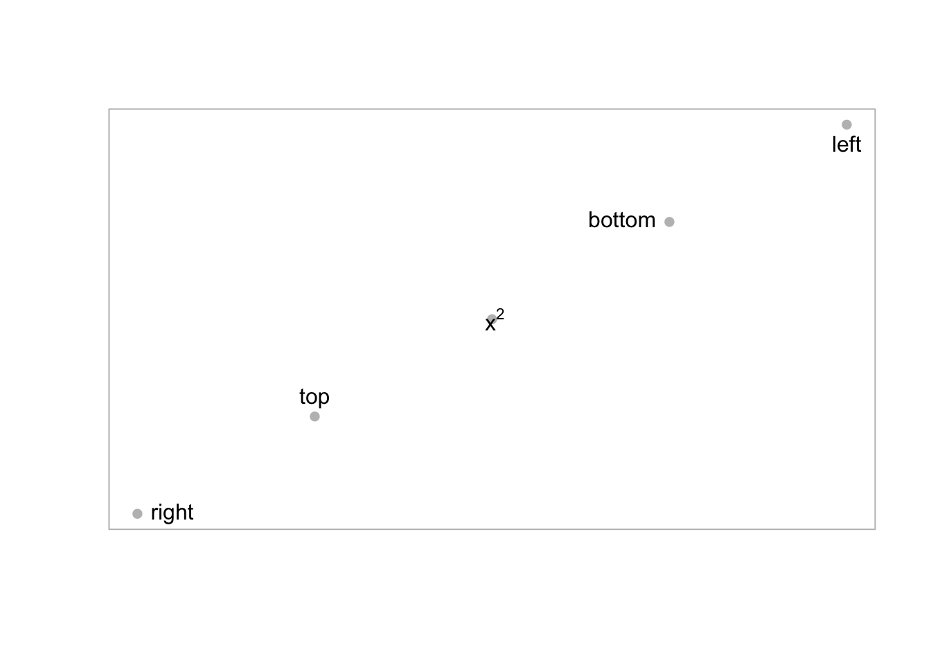
上述处理的都是向量数据,而matplot()、matpoints() 和 matlines()都是处理矩阵形式数据的。
绘图工具
grid() 可以添加网格线; abline() 添加直线; box() 在图形周围绘制矩形;rug() 可以沿着坐标轴绘制“地毯”图。
x = runif(20, 1, 10)
y = x + rnorm(20)
plot(x, y, ann=F, axes=F, col="gray", pch=16)
box(col="gray")

lmfit = lm(y ~ x)
abline(lmfit)
arrows(5, 8, 7, predict(lmfit, data.frame(x=7)),
       length = 0.1)
text(5, 8, "Line of best fit", pos = 2)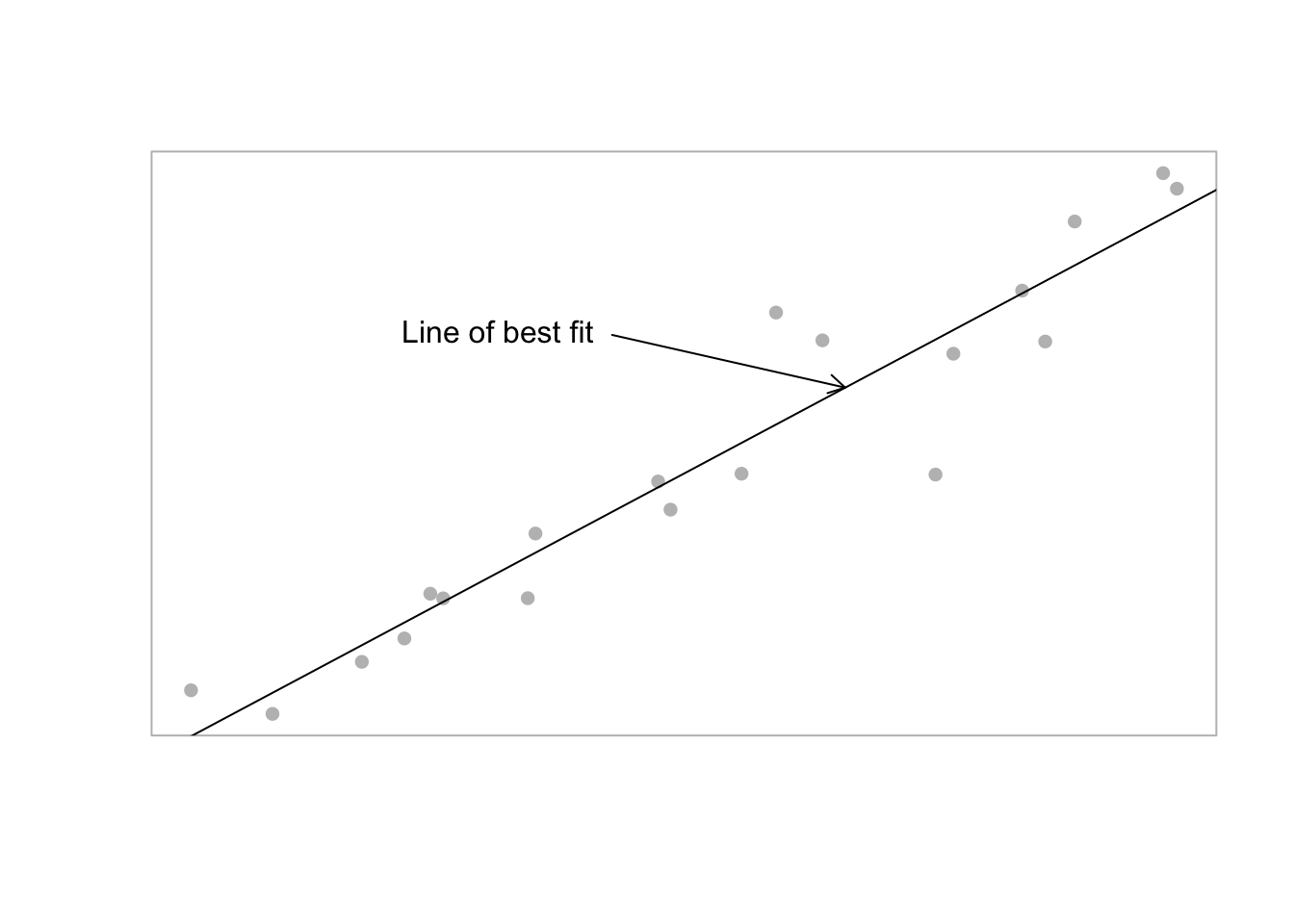
y = rnorm(50)
hist(y, main="", xlab="", ylab="", axes=F, border="gray", col="light gray")
box(col="gray")
rug(y, ticksize = 0.02)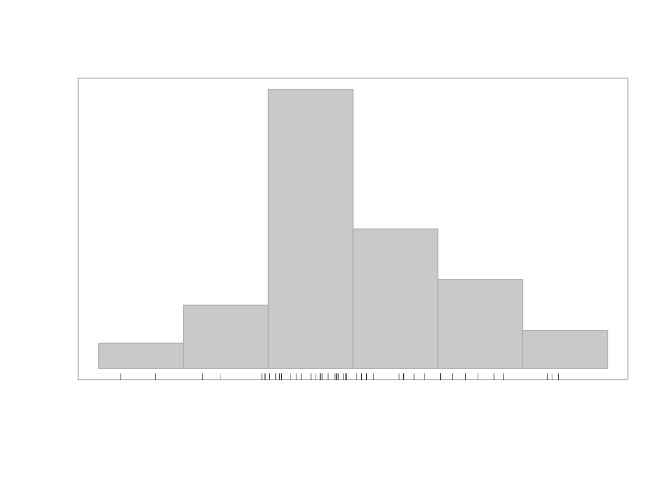
在边缘处添加图形
mtext() 函数可以在边缘区域的任何位置绘制文本,它的 outer 参数控制是在图像区域还是外部区域的边缘处输出。
side 控制在哪个边缘区域输出,1 - 底部,2 - 左侧,3 - 顶部,4 - 右侧。
我们也可以在图像区域或外部区域使用一般在绘图区域使用的函数,不过有点麻烦。我们需要先设定 xpd 的状态。
下面展示了一个例子:将绘制出的一个在两个图像之间穿越的矩形。
y1 = rnorm(100)
y2 = rnorm(100)

par(mfrow=c(2,1), xpd =NA)

# 绘制第一个图形
plot(y1, type="l", axes=FALSE,
     xlab="", ylab="", main="")
box(col="gray")
mtext("Left end of margin", adj=0, side=3)
lines(x=c(20,20,40,40), y=c(-7, max(y1), max(y1), -7), lwd=3, col="gray")

# 绘制第二个图形
plot(y2, type="l", axes=FALSE,
     xlab="", ylab="", main="")
box(col="gray")
mtext("Right end of margin", adj=1, side=3)
lines(x=c(20, 20, 40, 40), y=c(7, min(y2), min(y2), 7),
      lwd=3, col="gray")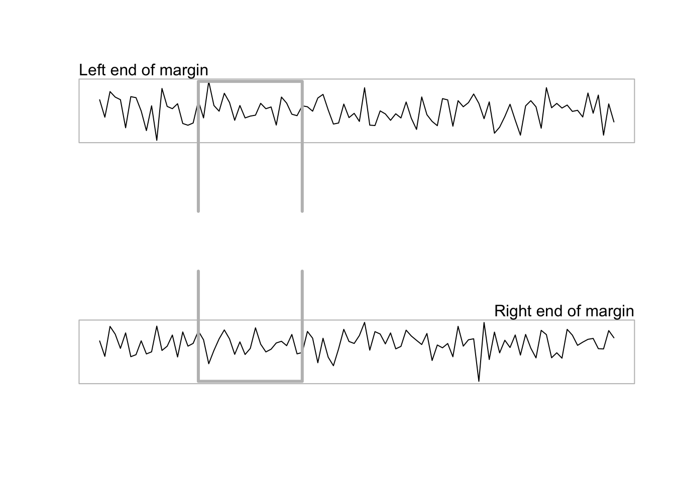
图例
legend() 函数用于在图像中添加图例或关键字。
第一个例子展示在散点图中添加图例的方法,图例将不同的组名和对应的符号关联起来。前 2 个参数给定对于用户坐标系统,
图例左上角的为止。第 3 个参数提供图例需要的标签,此外,通过指定 pch 参数可以在标签旁边绘制符号。
with(iris,
     plot(Sepal.Length, Sepal.Width, pch=as.numeric(Species), cex=1.2))
legend(6.1, 4.4, c("setosa", "versicolor", "virginica"),
       cex=1.5, pch=1:3)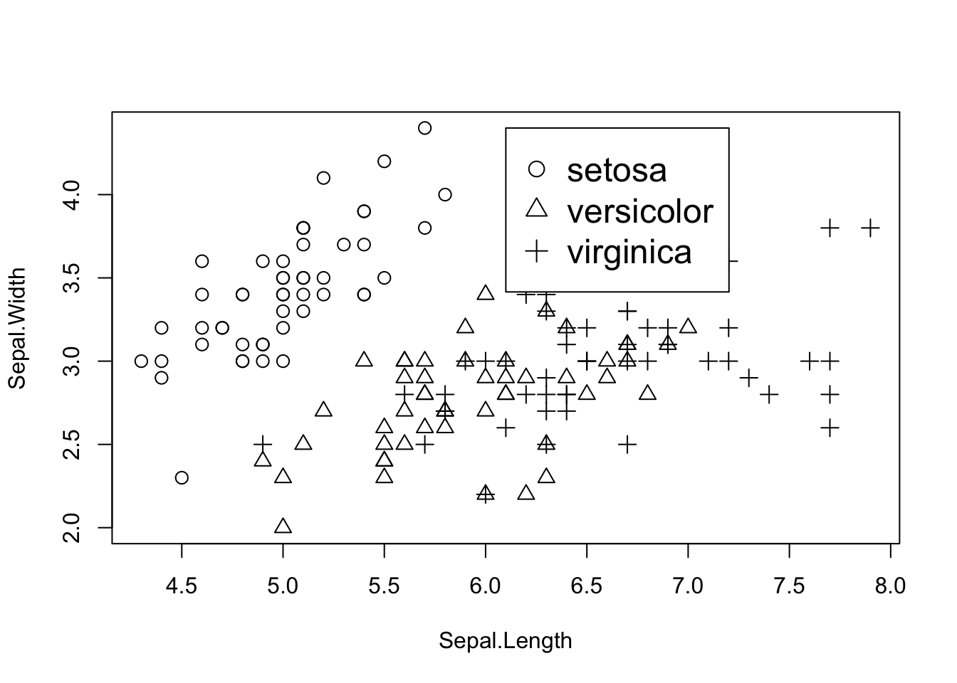
下一个例子展示条形图添加图例,图例中组名对应不同的填充模式。
barplot(VADeaths[1:2, ], angle = c(45, 135), density = 20,
        col="gray", names = c("RM", "RF", "UM", "UF"))
legend(0.4, 38, c("55-59", "50-54"), cex=1.5, angle = c(135, 45), density = 20, fill = "gray")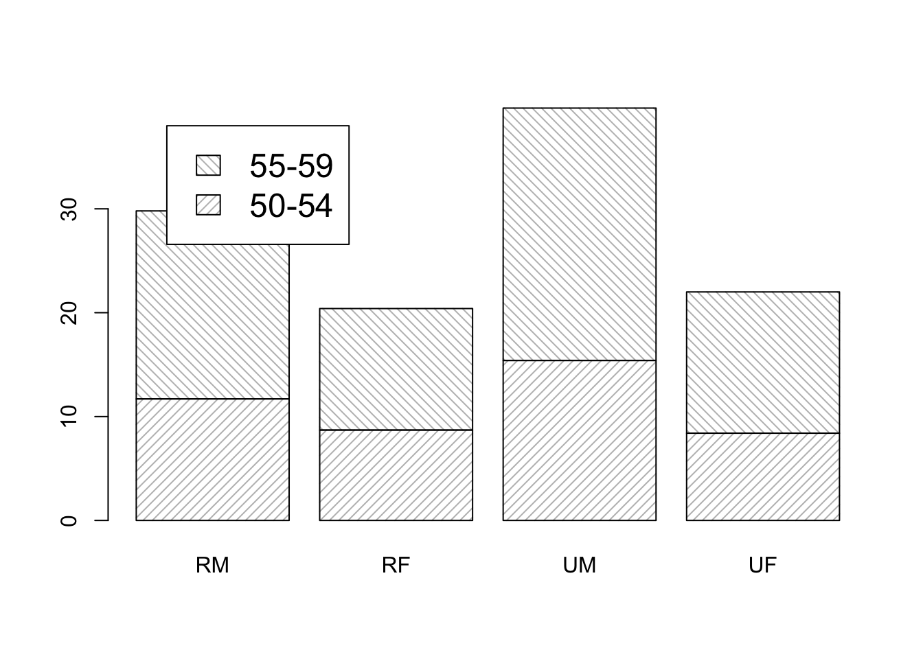
注意,怎么将图例符号对应于图形完全是由用户控制的。所以在绘制时一定要额外注意,相比于传统图形绘制, ggplot2 和 lattice 包会自动映射,更为方便。
坐标轴
有时候我们想要修改坐标轴,我们第一步需要禁止生成默认的坐标轴,这一点可以通过设置大多数高级函数的
axes 参数实现。 通过 par() 指定 xaxt = "n" 和 yaxt = "n" 也可以实现该目的。
下面举一个定制坐标轴的例子:
开始绘制一个初始图形,并且绘制 y 轴的尺度是摄氏度。接下来再绘制一个华氏温度的 y 轴。x 轴使用特殊标签,而不是默认刻度线的数值位置。
# 先生成数据并绘制没有数据符号和坐标轴的空图
x = 1:2
y = runif(2, 0, 100)
par(mar=c(4, 4, 2, 4))
plot(x, y, type = "n", xlim = c(0.5, 2.5), ylim = c(-10, 110),
     axes=FALSE, ann=FALSE)

# 指定主 y 轴摄氏度刻度位置。
axis(2, at=seq(0, 100, 20))  # 2 表示绘制在左边,at指定刻度线位置
mtext("Temperature (Centigrade)", side = 2, line = 3)

# 绘制有特殊标签的底部坐标轴,以及表示华氏温度的 y 轴
axis(1, at=1:2, labels = c("Treatment1", "Treatment2"))
axis(4, at=seq(0, 100, 20), labels = seq(0, 100, 20)*9/5 + 32)
mtext("Temperature (Fahrenheit)", side=4, line=3)
box()

# 最后画一些温度样式的符号表示实际温度
segments(x, 0, x, 100, lwd=20)
segments(x, 0, x, 100, lwd=16, col="white")
segments(x, 0, x, y, lwd = 16, col = "gray")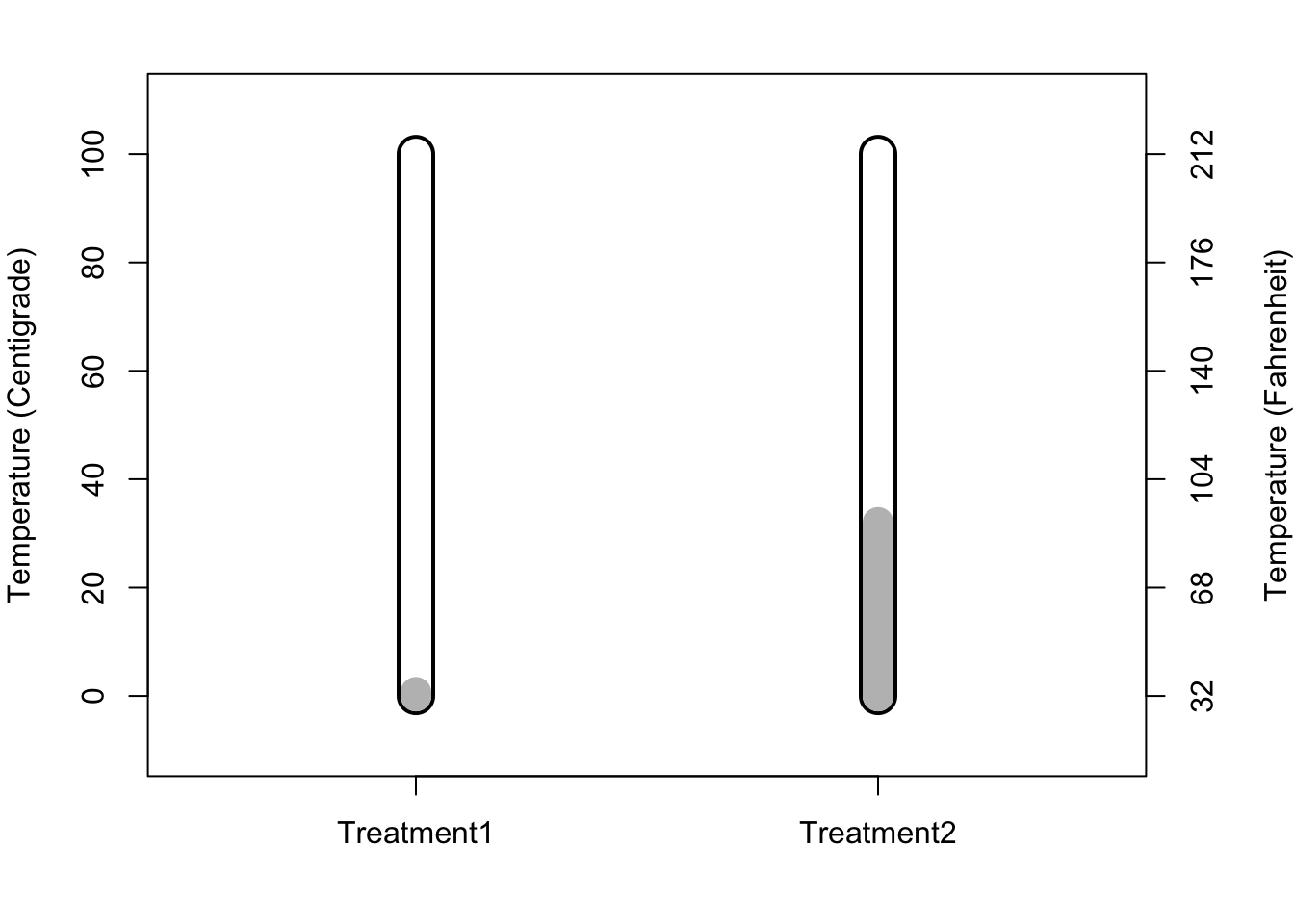
坐标系统
在绘图区域内的图形输出是根据坐标轴的尺度自动定位的,而图形边缘处的文本则是根据距离绘图区域边界多少 文本行定位的。
par() 函数
一般情况下我们使用 par() 函数获取或设定图形的状态。其中 din、fin和pin 3个状态反映了当前绘图设备、图像区域以及回去区域的尺寸(宽度和高度),以英寸为单位。
par("din")
#> [1] 7 5
par("fin")
#> [1] 7 5
par("pin")
#> [1] 5.76 3.16
usr 反映坐标轴范围。
par("usr")
#> [1] 0 1 0 1
下面我们画一把与实际物理尺寸对应的尺子。
# 绘制一个空白图形并进行计算
plot(0:1, 0:1, type="n", axes=F, ann=F)
usr = par("usr")
pin = par("pin")
xcm = diff(usr[1:2])/(pin[1]*2.54)
ycm = diff(usr[3:4])/(pin[2]*2.54)

# 现在绘制的图形是根据厘米表示的
par(xpd=NA)
rect(0 + 0.2*xcm, 0-0.2*ycm,
1 + 0.2*xcm, 0.3-0.2*ycm,
col="gray", border = NA)

# 绘制边框、刻度和标签
rect(0, 0, 1, 0.3, col="white")
segments(seq(1, 8, 0.1)*xcm, 0,
seq(1, 8, 0.1)*xcm,
c(rep(c(0.5,
rep(0.25, 4),
0.35,
rep(0.25, 4)), 7),
0.5)*ycm)
text(1:8*xcm, 0.6*ycm, 0:7, adj=c(0.5, 0))
text(8.2*xcm, 0.6*ycm, "cm", adj=c(0, 0))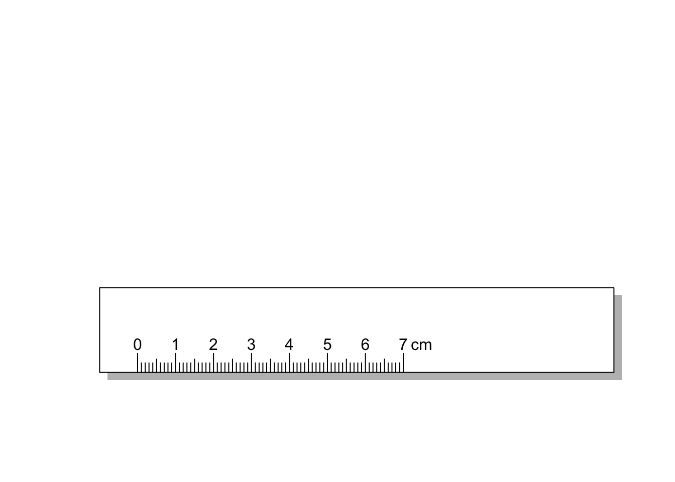
覆盖输出
有时在同一图中绘制 2 个数据集非常有用,此时数据集共享一个 x 变量,但拥有不同的 y 尺度。
至少有 2 种方法:
- 调用
par(new=TRUE)实现 2 个不同图形在彼此之上重叠绘制 - 在绘制第二个数据之前显式地重置
usr状态
方法一
drunkness = ts(c(3875, 4846, 5128, 5773, 7327,
                 6688, 5582, 3473, 3186, rep(NA, 51)),
               start = 1912, end = 1971)

par(mar = c(5, 6, 2, 4))
plot(drunkness, lwd=3, col="gray", ann=F, las=2)
mtext("Drunkness\nRelated Arrest", side=2, line=3.5)
par(new=TRUE)
plot(nhtemp, ann=F, axes=F)
mtext("Temperature (F)", side=4, line=3)
title("Using par(new=TRUE)")
axis(4)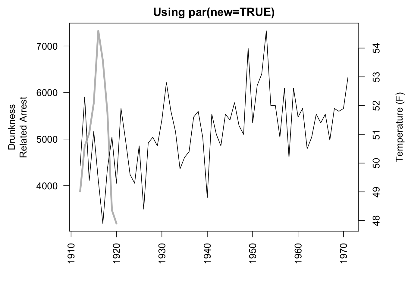
方法二
该方法只绘制一个图形。
par(mar=c(5, 6, 2, 4))
plot(drunkness, lwd=3, col="gray", ann=F, las=2)
mtext("Drunkness\nRelated Arrest", side=2, line=3.5)
usr = par("usr")
par(usr=c(usr[1:2], 47.6, 54.9))
lines(nhtemp)
mtext("Temperature (F)", side=4, line=3)
title("Using par(usr=...)")
axis(4)
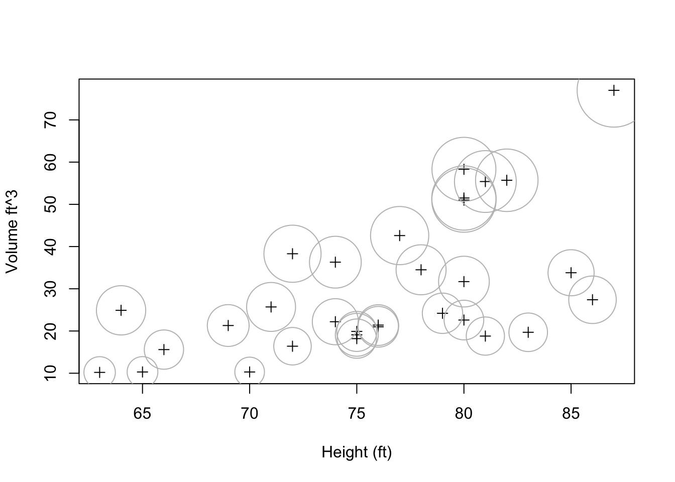
方法三
一些高级函数提供了一个叫 add 的参数,如果设置为 TRUE,将会在现有图形上添加输出。
with(trees,
     expr = {
     plot(Height, Volume, pch=3, xlab="Height (ft)",
          ylab=expression(paste("Volume ", "ft^3")))
     symbols(Height, Volume, circles = Girth/12,
             fg="gray", inches = FALSE, add=TRUE)
       })
特殊情况
隐藏的坐标轴尺度
因为这个原因,在条形图和箱线图中添加图形输出会比较麻烦。为何做到这点,我们需要获取函数的返回值。这个值会给出函数绘制的每一个条形的中点 x 位置。
条形图例子:添加水平参考线段
y = sample(1:10)
midpts = barplot(y, col="lightgray")
width = diff(midpts[1:2])/4
left = rep(midpts, y - 1) - width
right = rep(midpts, y - 1) + width
heights = unlist(apply(matrix(y, ncol=10),
                       2, seq))[-cumsum(y)]
segments(left, heights, right, heights,
         col="white")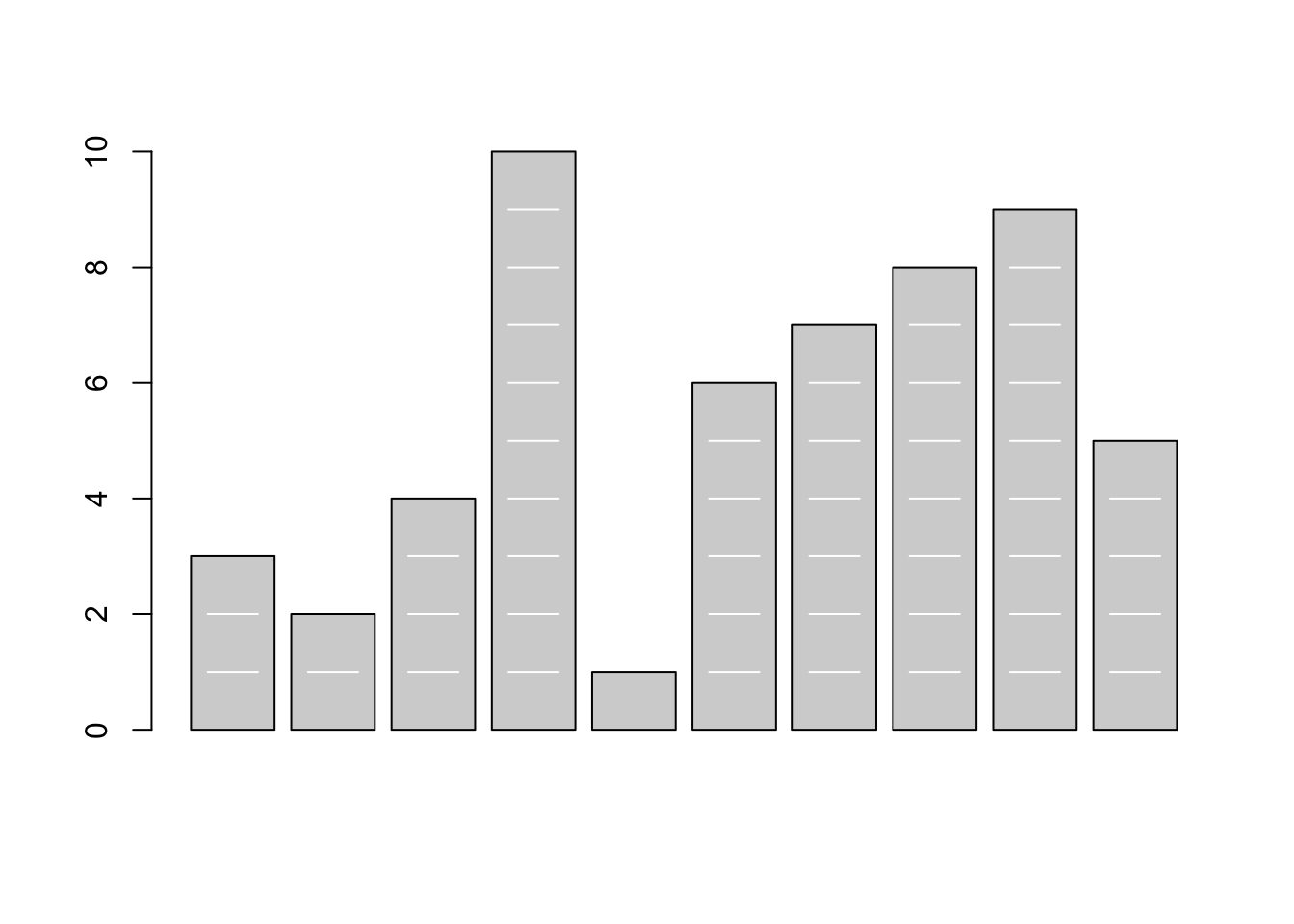
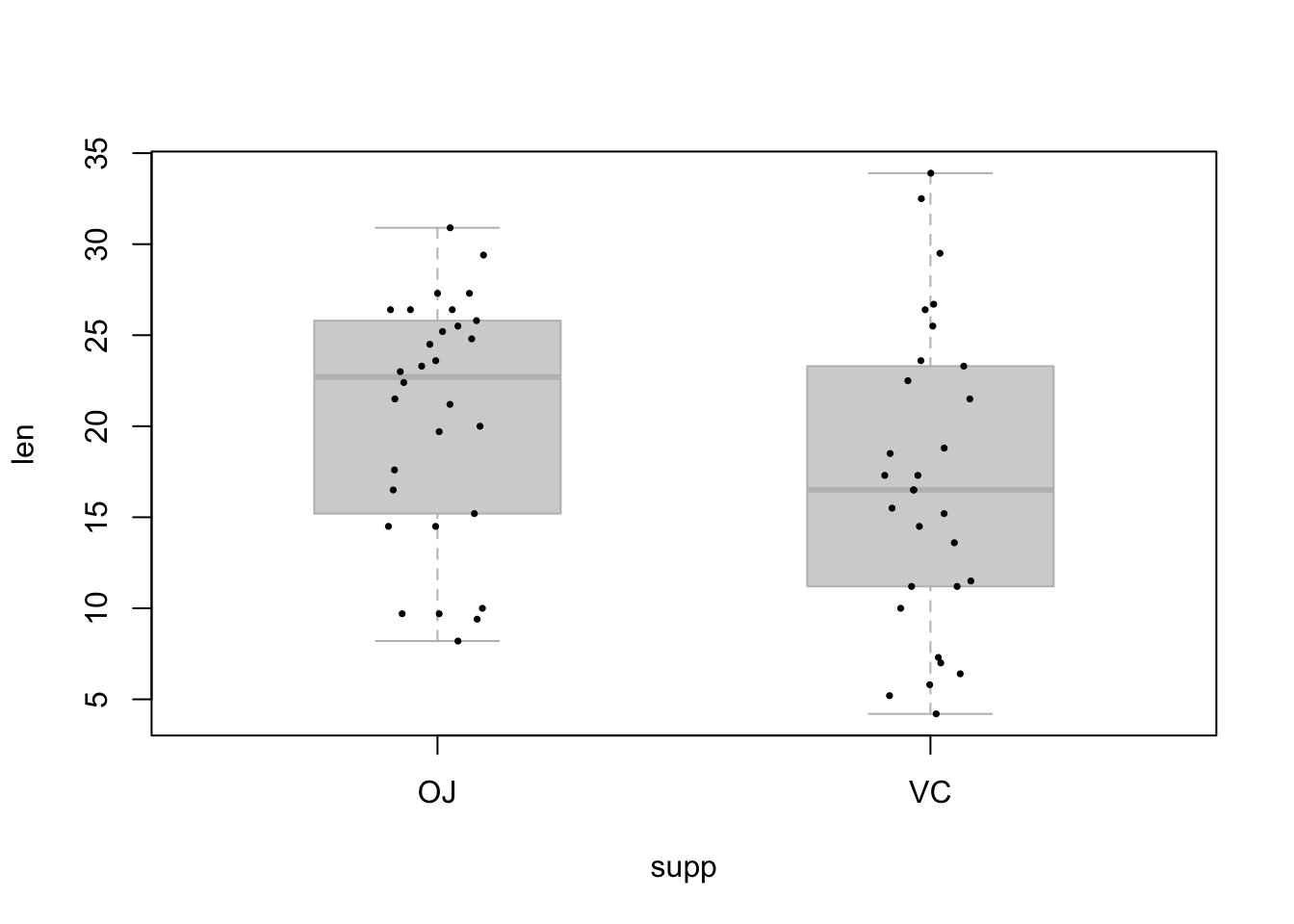
箱线图例子:添加抖动点
with(ToothGrowth,
     {
       boxplot(len ~ supp, border = "gray",
               col="lightgray", boxwex=0.5)
       points(jitter(rep(1:2, each=30), 0.5),
              unlist(split(len, supp)),
              cex=0.5, pch=16)
     })
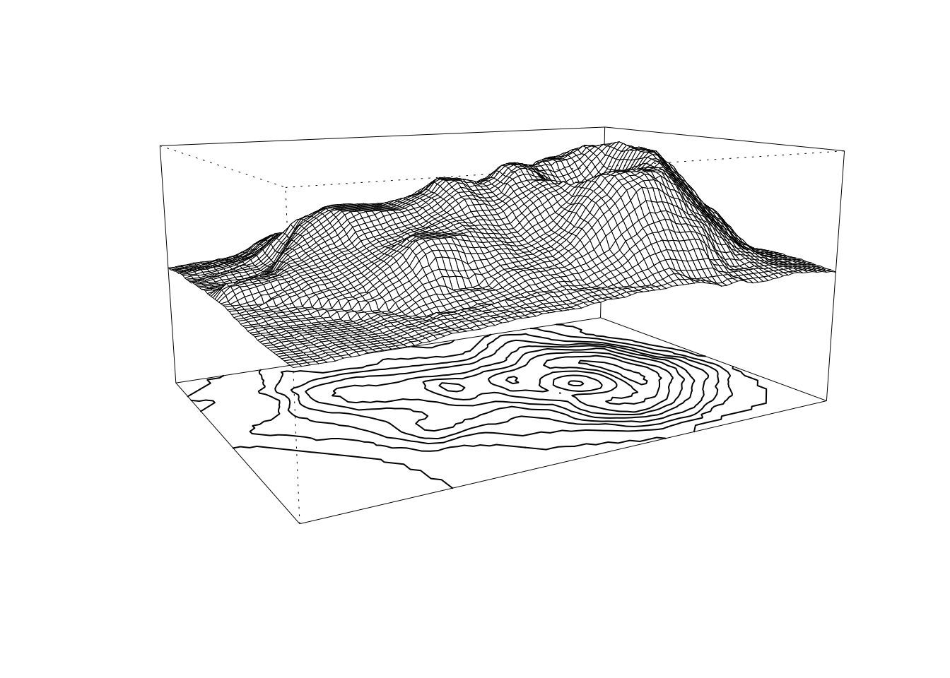
绘制三维图像
添加图像步骤:
- 获取
persp()函数返回的变换矩阵 (本身该函数会绘制三维图像) - 使用
trans3d()函数将三维位置转换为二位位置 - 将以上结果传给标准函数,如
lines()、text()
下面绘制火山并添加等高线。
z = 2*volcano
x = 10 * (1:nrow(z))
y = 10 * (1:ncol(z))

trans = persp(x, y, z, zlim=c(0, max(z)),
              theta=150, phi=12, lwd=.5,
              scale=F, axes=F)

# 计算等高线
clines = contourLines(x, y, z)
# 将等高线 x 与 y 顶点位置传给 trans3d()
lapply(clines,
       function(contour) {
         lines(trans3d(contour$x, contour$y, 0, trans))
       })
#> [[1]]
#> NULL
#>
#> [[2]]
#> NULL
#>
#> [[3]]
#> NULL
#>
#> [[4]]
#> NULL
#>
#> [[5]]
#> NULL
#>
#> [[6]]
#> NULL
#>
#> [[7]]
#> NULL
#>
#> [[8]]
#> NULL
#>
#> [[9]]
#> NULL
#>
#> [[10]]
#> NULL
#>
#> [[11]]
#> NULL
#>
#> [[12]]
#> NULL
#>
#> [[13]]
#> NULL
#>
#> [[14]]
#> NULL
#>
#> [[15]]
#> NULL
#>
#> [[16]]
#> NULL
#>
#> [[17]]
#> NULL
#>
#> [[18]]
#> NULL
#>
#> [[19]]
#> NULL
#>
#> [[20]]
#> NULL
创建新图形
plot.new() 函数开启一个新的绘图(与 frame() 等价),并将 x 与 y 尺度设置为 (0, 1) 区间。
plot.window() 函数重置用户坐标系统的尺度。
plot.xy() 在绘图区域绘制数据符号和线条。
从头创建一个简单图形
plot.new()  # 开启一个空白绘图
plot.window(range(pressure$temperature),
            range(pressure$pressure))  # 设定坐标轴尺度
plot.xy(pressure, type="p")  # 绘制图形
box()  # 围绕绘图区域绘制矩形
axis(1) # 添加轴线
axis(2) # 添加轴线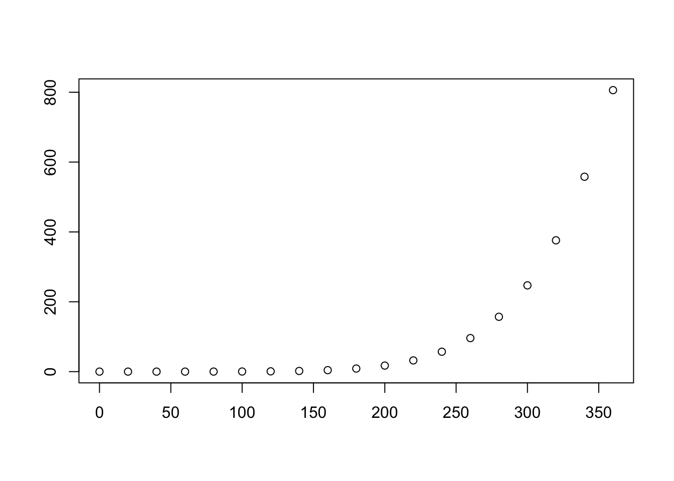
这和 plot() 绘制的散点图完全一致。
从头创建一个复杂图形
绘制泰坦尼克号成年男性和女性幸存者数目。
groups = dimnames(Titanic)[[1]]
males = Titanic[, 1, 2, 2]
females = Titanic[, 2, 2, 2]

males
#>  1st  2nd  3rd Crew
#>   57   14   75  192
females
#>  1st  2nd  3rd Crew
#>  140   80   76   20
# 6 行内容,4行用户绘制条形,1行用于绘制x轴,1行绘制图例(-1)
par(mar=c(0.5, 3, 0.5, 1))
plot.new()
plot.window(xlim = c(-200,200), ylim = c(-1.5, 4.5))
ticks = seq(-200, 200, 100)
y = 1:4
h = 0.2
# 开始画图
# x 轴绘制在绘图区域内部(设置pos=0)
lines(rep(0,2), c(-1.5, 4.5), col="gray")
segments(-200, y, 200, y, lty = "dotted")
rect(-males, y-h, 0, y+h, col="darkgray")
rect(0, y-h, females, y+h, col="lightgray")
mtext(groups, at=y, adj=1, side=2, las=2)
par(cex.axis=0.5, mex=0.5)
axis(1, at=ticks, labels=abs(ticks), pos=0)
# 在底部绘制图例
# 确保矩形能包含文字
tw = 1.5*strwidth("females")
rect(-tw, -1-h, 0, -1+h, col="darkgray")
rect(0, -1-h, tw, -1+h, col="lightgray")
text(0, -1, "males", pos=2)
text(0, -1, "females", pos=4)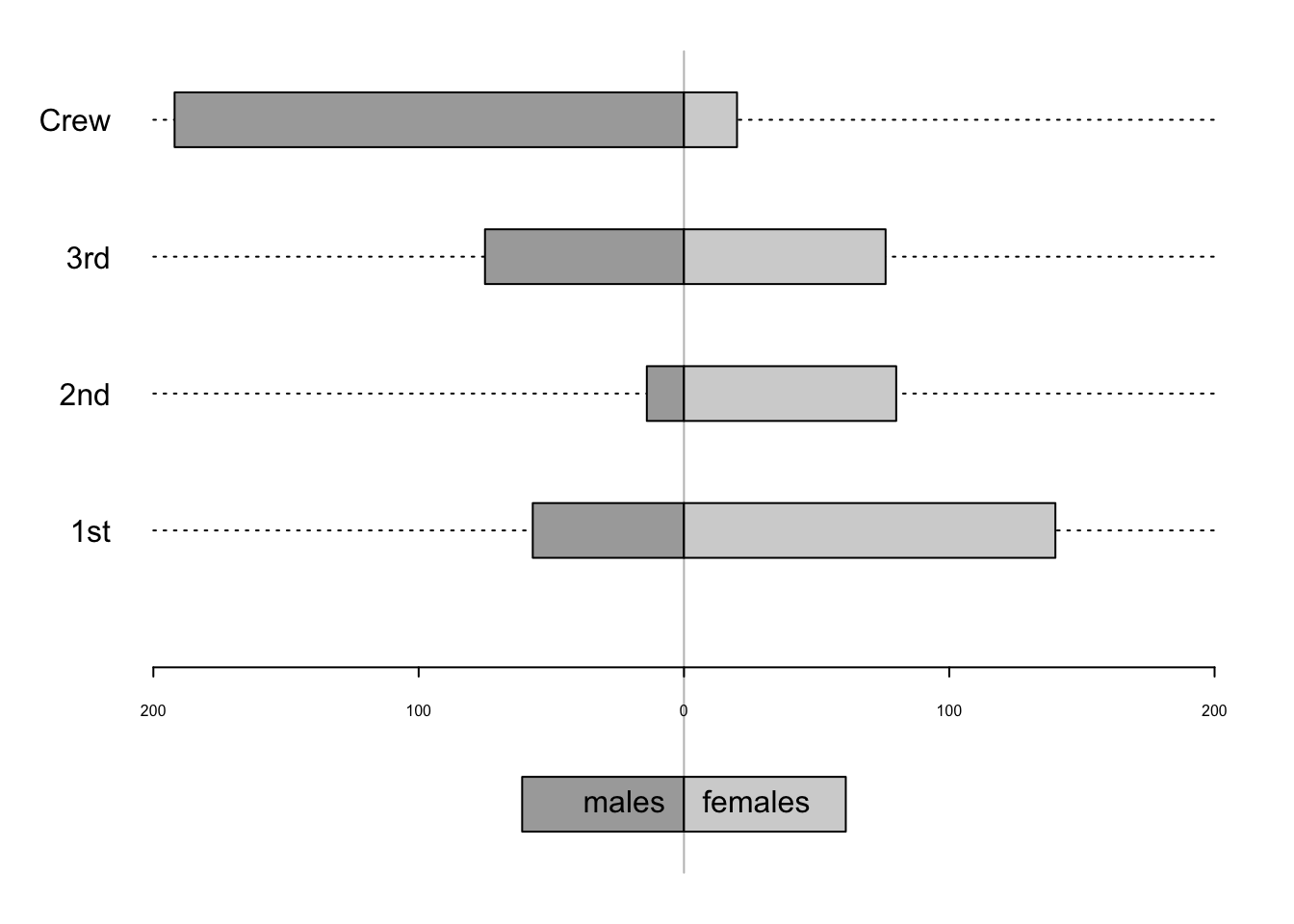
创建绘图函数
xy.coords()允许在新建的函数中灵活指定 x 与 y 参数。该函数接收 x 参数与 y 参数并且创建一个标准的包含 x 值、y 值以及坐标轴合理标签的对象。
一个新的绘图函数可能需要强制将 xpd 状态设定为 NA,从而在绘图区域外绘制线条和文本。这种情况下可以在函数的末尾恢复初始的绘图状态。
可以采用以下技术:
# 放在函数的开始部分
opar = par(no.readonly = TRUE)
on.exit(par(opar))
下面是一个绘图模板(可以看做 plot() 函数的精简版本),提供了一个供他人使用的绘图函数的出发点。
plot.newclass =
  function(x, y=NULL,
           main="", sub="",
           xlim=NULL, ylim=NULL,
           axes=TRUE, ann=par("ann"),
           col=par("col"),
           ...) {
    xy = xy.coords(x, y)
    if (is.null(xlim)) {
      xlim = range(xy$x[is.finite(xy$x)])
    }
    if (is.null(ylim)) {
      ylim = range(xy$y[is.finite(xy$y)])
    }
    opar = par(no.readonly = TRUE)
    on.exit(par(opar))
    plot.new()
    plot.window(xlim, ylim, ...)
    points(xy$x, xy$y, col=col, ...)
    if (axes) {
      axis(1)
      axis(2)
      box()
    }
    if (ann) {
      title(main=main, sub=sub, xlab=xy$xlab, ylab=xy$ylab, ...)
    }
           }
资料:《R绘图系统》(第二版)