管道统计分析——rstatix使用指南
王诗翔 · 2019-07-07
原英文文档地址:https://raw.githubusercontent.com/kassambara/rstatix/master/README.Rmd
rstatix 包提供了一个与「tidyverse」设计哲学一致的简单且直观的管道友好框架用于执行基本的统计检验, 包括 t 检验、Wilcoxon 检验、ANOVA、Kruskal-Wallis 以及相关分析。
每个检验的输出都会自动转换为干净的数据框以便于可视化。
另外也提供了一些用于重塑、重排、操作以及可视化相关矩阵的函数。也包含一些方便因子实验分析的函数,包括 ‘within-Ss’ 设计 (repeated measures), purely ‘between-Ss’ 设计以及 mixed ‘within-and-between-Ss’ 设计。
该包也可以用于计算一些效应值度量,包括 “eta squared” for ANOVA, “Cohen’s d” for t-test and “Cramer’s V” for the association between categorical variables。 该包还包含一些用于识别单变量和多变量离群点、评估变异正态性和异质性的帮助函数。
核心函数
描述统计量
get_summary_stats(): Compute summary statistics for one or multiple numeric variables. Can handle grouped data.freq_table(): Compute frequency table of categorical variables.get_mode(): Compute the mode of a vector, that is the most frequent values.identify_outliers(): Detect univariate outliers using boxplot methods.mahalanobis_distance(): Compute Mahalanobis Distance and Flag Multivariate Outliers.shapiro_test()andmshapiro_test(): Univariate and multivariate Shapiro-Wilk normality test.
比较均值
t_test(): perform one-sample, two-sample and pairwise t-testswilcox_test(): perform one-sample, two-sample and pairwise Wilcoxon testssign_test(): perform sign test to determine whether there is a median difference between paired or matched observations.anova_test(): an easy-to-use wrapper aroundcar::Anova()to perform different types of ANOVA tests, including independent measures ANOVA, repeated measures ANOVA and mixed ANOVA.kruskal_test(): perform kruskal-wallis rank sum testtukey_hsd(): performs tukey post-hoc tests. Can handle different inputs formats: aov, lm, formula.dunn_test(): compute multiple pairwise comparisons following Kruskal-Wallis test.emmeans_test(): pipe-friendly wrapper arroundemmeansfunction to perform pairwise comparisons of estimated marginal means. Useful for post-hoc analyses following up ANOVA/ANCOVA tests.get_comparisons(): Create a list of possible pairwise comparisons between groups.get_pvalue_position: autocompute p-value positions for plotting significance using ggplot2.
促进R的ANOVA计算
factorial_design(): build factorial design for easily computing ANOVA using thecar::Anova()function. This might be very useful for repeated measures ANOVA, which is hard to set up with thecarpackage.anova_summary(): Create beautiful summary tables of ANOVA test results obtained from eithercar::Anova()orstats::aov(). The results include ANOVA table, generalized effect size and some assumption checks, such as Mauchly’s test for sphericity in the case of repeated measures ANOVA.
比较方差
levene_test(): Pipe-friendly framework to easily compute Levene’s test for homogeneity of variance across groups. Handles grouped data.box_m(): Box’s M-test for homogeneity of covariance matrices
效应值
cohens_d(): Compute cohen’s d measure of effect size for t-tests.eta_squared()andpartial_eta_squared(): Compute effect size for ANOVA.cramer_v(): Compute Cramer’s V, which measures the strength of the association between categorical variables.
相关分析
计算相关性:
cor_test(): correlation test between two or more variables using Pearson, Spearman or Kendall methods.cor_mat(): compute correlation matrix with p-values. Returns a data frame containing the matrix of the correlation coefficients. The output has an attribute named “pvalue”, which contains the matrix of the correlation test p-values.cor_get_pval(): extract a correlation matrix p-values from an object of classcor_mat().cor_pmat(): compute the correlation matrix, but returns only the p-values of the correlation tests.as_cor_mat(): convert acor_testobject into a correlation matrix format.
重塑相关矩阵:
cor_reorder(): reorder correlation matrix, according to the coefficients, using the hierarchical clustering method.cor_gather(): takes a correlation matrix and collapses (or melt) it into long format data frame (paired list)cor_spread(): spread a long correlation data frame into wide format (correlation matrix).
取子集:
cor_select(): subset a correlation matrix by selecting variables of interest.pull_triangle(),pull_upper_triangle(),pull_lower_triangle(): pull upper and lower triangular parts of a (correlation) matrix.replace_triangle(),replace_upper_triangle(),replace_lower_triangle(): replace upper and lower triangular parts of a (correlation) matrix.
可视化相关矩阵:
cor_as_symbols(): replaces the correlation coefficients, in a matrix, by symbols according to the value.cor_plot(): visualize correlation matrix using base plot.cor_mark_significant(): add significance levels to a correlation matrix.
矫正p值和添加显著性标记
adjust_pvalue(): add an adjusted p-values column to a data frame containing statistical test p-valuesadd_significance(): add a column containing the p-value significance level
其他
doo(): alternative to dplyr::do for doing anything. Technically it usesnest() + mutate() + map()to apply arbitrary computation to a grouped data frame.sample_n_by(): sample n rows by group from a tableconvert_as_factor(), set_ref_level(), reorder_levels(): Provides pipe-friendly functions to convert simultaneously multiple variables into a factor variable.make_clean_names(): Pipe-friendly function to make syntactically valid column names (for input data frame) or names (for input vector).
安装和加载
- 从GitHub上安装开发版本:
if(!require(devtools)) install.packages("devtools")
devtools::install_github("kassambara/rstatix")- 或者从CRAN安装稳定版本:
install.packages("rstatix")- 加载包
library(rstatix)
#>
#> Attaching package: 'rstatix'
#> The following object is masked from 'package:stats':
#>
#>     filter
library(ggpubr)  # For easy data-visualization
#> Loading required package: ggplot2
描述统计量
# Summary statistics of some selected variables
#::::::::::::::::::::::::::::::::::::::::::::::::::::::::::
iris %>%
  get_summary_stats(Sepal.Length, Sepal.Width, type = "common")
#> # A tibble: 2 x 10
#>   variable         n   min   max median   iqr  mean    sd    se    ci
#>   <chr>        <dbl> <dbl> <dbl>  <dbl> <dbl> <dbl> <dbl> <dbl> <dbl>
#> 1 Sepal.Length   150   4.3   7.9    5.8   1.3  5.84 0.828 0.068 0.134
#> 2 Sepal.Width    150   2     4.4    3     0.5  3.06 0.436 0.036 0.07

# Whole data frame
#::::::::::::::::::::::::::::::::::::::::::::::::::::::::::
iris %>% get_summary_stats(type = "common")
#> # A tibble: 4 x 10
#>   variable         n   min   max median   iqr  mean    sd    se    ci
#>   <chr>        <dbl> <dbl> <dbl>  <dbl> <dbl> <dbl> <dbl> <dbl> <dbl>
#> 1 Petal.Length   150   1     6.9   4.35   3.5  3.76 1.76  0.144 0.285
#> 2 Petal.Width    150   0.1   2.5   1.3    1.5  1.20 0.762 0.062 0.123
#> 3 Sepal.Length   150   4.3   7.9   5.8    1.3  5.84 0.828 0.068 0.134
#> 4 Sepal.Width    150   2     4.4   3      0.5  3.06 0.436 0.036 0.07


# Grouped data
#::::::::::::::::::::::::::::::::::::::::::::::::::::::::::
iris %>%
  group_by(Species) %>%
  get_summary_stats(Sepal.Length, type = "mean_sd")
#> # A tibble: 3 x 5
#>   Species    variable         n  mean    sd
#>   <fct>      <chr>        <dbl> <dbl> <dbl>
#> 1 setosa     Sepal.Length    50  5.01 0.352
#> 2 versicolor Sepal.Length    50  5.94 0.516
#> 3 virginica  Sepal.Length    50  6.59 0.636
比较均值
你可以使用 t_test() (parametric) or wilcox_test() (non-parametric,实际比较的是中位数) 比较均值差异。下面使用 t 检验进行示范。
数据
导入样例数据集:
df <- ToothGrowth
df$dose <- as.factor(df$dose)
head(df)
#>    len supp dose
#> 1  4.2   VC  0.5
#> 2 11.5   VC  0.5
#> 3  7.3   VC  0.5
#> 4  5.8   VC  0.5
#> 5  6.4   VC  0.5
#> 6 10.0   VC  0.5
比较2个独立组别
- 创建一个带p值的箱线图
# T-test
stat.test <- df %>%
  t_test(len ~ supp, paired = FALSE)
stat.test
#> # A tibble: 1 x 8
#>   .y.   group1 group2    n1    n2 statistic    df      p
#> * <chr> <chr>  <chr>  <int> <int>     <dbl> <dbl>  <dbl>
#> 1 len   OJ     VC        30    30      1.92  55.3 0.0606

# Create a box plot
p <- ggboxplot(
  df, x = "supp", y = "len",
  color = "supp", palette = "jco", ylim = c(0,40)
  )
# Add the p-value manually
p + stat_pvalue_manual(stat.test, label = "p", y.position = 35)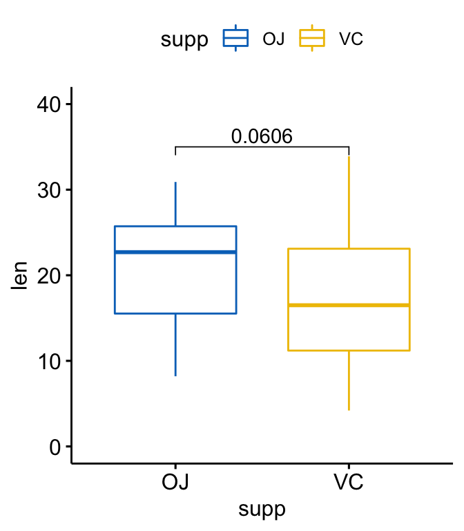
- 使用 glue expression 自定义标签:
p +stat_pvalue_manual(stat.test, label = "T-test, p = {p}",
                      y.position = 36)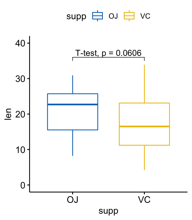
- 分组数据:在按照「dose」分组后比较 supp 水平:
# Statistical test
stat.test <- df %>%
  group_by(dose) %>%
  t_test(len ~ supp) %>%
  adjust_pvalue() %>%
  add_significance("p.adj")
stat.test
#> # A tibble: 3 x 11
#>   dose  .y.   group1 group2    n1    n2 statistic    df       p   p.adj
#>   <fct> <chr> <chr>  <chr>  <int> <int>     <dbl> <dbl>   <dbl>   <dbl>
#> 1 0.5   len   OJ     VC        10    10    3.17    15.0 0.00636 0.0127
#> 2 1     len   OJ     VC        10    10    4.03    15.4 0.00104 0.00312
#> 3 2     len   OJ     VC        10    10   -0.0461  14.0 0.964   0.964
#> # ... with 1 more variable: p.adj.signif <chr>

# Visualization
ggboxplot(
  df, x = "supp", y = "len",
  color = "supp", palette = "jco", facet.by = "dose",
  ylim = c(0, 40)
  ) +
  stat_pvalue_manual(stat.test, label = "p.adj", y.position = 35)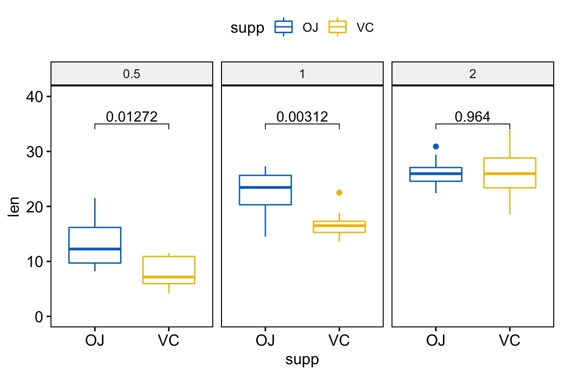
比较配对样本
# T-test
stat.test <- df %>%
  t_test(len ~ supp, paired = TRUE)
stat.test
#> # A tibble: 1 x 8
#>   .y.   group1 group2    n1    n2 statistic    df       p
#> * <chr> <chr>  <chr>  <int> <int>     <dbl> <dbl>   <dbl>
#> 1 len   OJ     VC        30    30      3.30    29 0.00255

# Box plot
p <- ggpaired(
  df, x = "supp", y = "len", color = "supp", palette = "jco",
  line.color = "gray", line.size = 0.4, ylim = c(0, 40)
  )
p + stat_pvalue_manual(stat.test, label = "p", y.position = 36)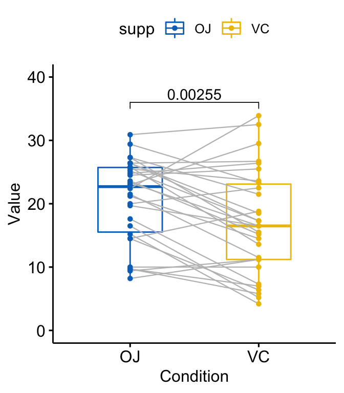
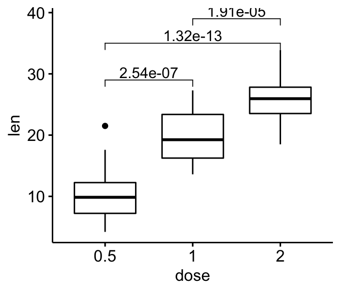
成对比较
- 成对比较:如果分组变量包含多于2个分类,会自动执行成对比较
# Pairwise t-test
pairwise.test <- df %>% t_test(len ~ dose)
pairwise.test
#> # A tibble: 3 x 10
#>   .y.   group1 group2    n1    n2 statistic    df        p    p.adj p.adj.signif
#> * <chr> <chr>  <chr>  <int> <int>     <dbl> <dbl>    <dbl>    <dbl> <chr>
#> 1 len   0.5    1         20    20     -6.48  38.0 1.27e- 7 2.54e- 7 ****
#> 2 len   0.5    2         20    20    -11.8   36.9 4.40e-14 1.32e-13 ****
#> 3 len   1      2         20    20     -4.90  37.1 1.91e- 5 1.91e- 5 ****
# Box plot
ggboxplot(df, x = "dose", y = "len")+
  stat_pvalue_manual(
    pairwise.test, label = "p.adj",
    y.position = c(29, 35, 39)
    )
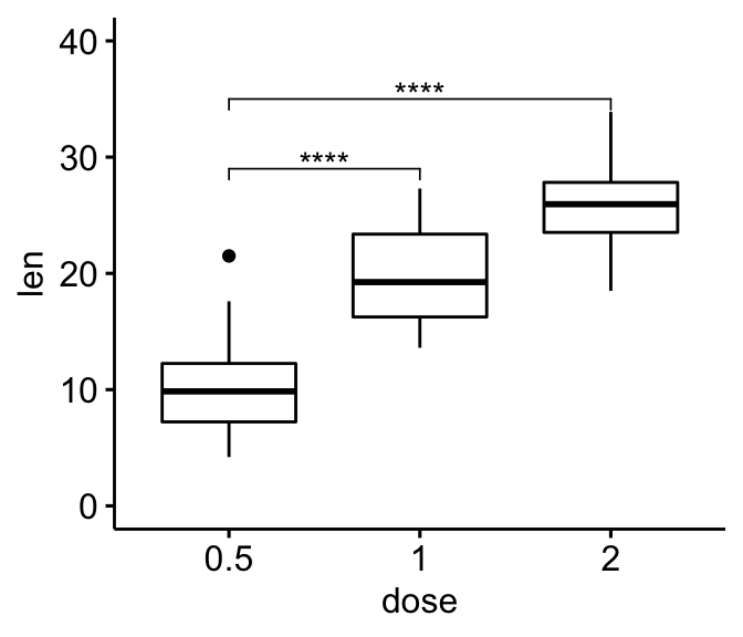
- 基于参考组的成对比较
# Comparison against reference group
#::::::::::::::::::::::::::::::::::::::::
# T-test: each level is compared to the ref group
stat.test <- df %>% t_test(len ~ dose, ref.group = "0.5")
stat.test
#> # A tibble: 2 x 10
#>   .y.   group1 group2    n1    n2 statistic    df        p    p.adj p.adj.signif
#> * <chr> <chr>  <chr>  <int> <int>     <dbl> <dbl>    <dbl>    <dbl> <chr>
#> 1 len   0.5    1         20    20     -6.48  38.0 1.27e- 7 1.27e- 7 ****
#> 2 len   0.5    2         20    20    -11.8   36.9 4.40e-14 8.80e-14 ****
# Box plot
ggboxplot(df, x = "dose", y = "len", ylim = c(0, 40)) +
  stat_pvalue_manual(
    stat.test, label = "p.adj.signif",
    y.position = c(29, 35)
    )
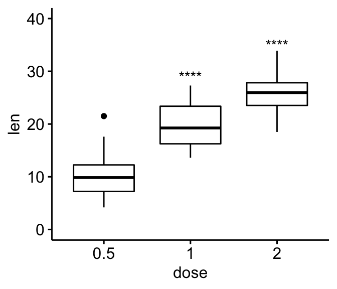
# Remove bracket
ggboxplot(df, x = "dose", y = "len", ylim = c(0, 40)) +
  stat_pvalue_manual(
    stat.test, label = "p.adj.signif",
    y.position = c(29, 35),
    remove.bracket = TRUE
    )
- 基于总体水平的成对比较
# T-test
stat.test <- df %>% t_test(len ~ dose, ref.group = "all")
stat.test
#> # A tibble: 3 x 10
#>   .y.   group1 group2    n1    n2 statistic    df         p   p.adj p.adj.signif
#> * <chr> <chr>  <chr>  <int> <int>     <dbl> <dbl>     <dbl>   <dbl> <chr>
#> 1 len   all    0.5       60    20     5.82   56.4   2.90e-7 8.70e-7 ****
#> 2 len   all    1         60    20    -0.660  57.5   5.12e-1 5.12e-1 ns
#> 3 len   all    2         60    20    -5.61   66.5   4.25e-7 8.70e-7 ****
# Box plot with horizontal mean line
ggboxplot(df, x = "dose", y = "len") +
  stat_pvalue_manual(
    stat.test, label = "p.adj.signif",
    y.position = 35,
    remove.bracket = TRUE
    ) +
  geom_hline(yintercept = mean(df$len), linetype = 2)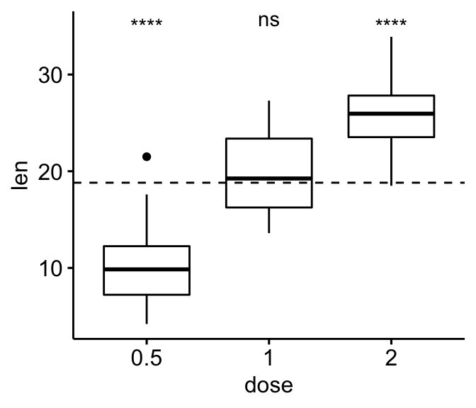
ANOVA 检验
# One-way ANOVA test
#:::::::::::::::::::::::::::::::::::::::::
df %>% anova_test(len ~ dose)
#> Coefficient covariances computed by hccm()
#> ANOVA Table (type II tests)
#>
#>   Effect DFn DFd    F        p p<.05   ges
#> 1   dose   2  57 67.4 9.53e-16     * 0.703

# Two-way ANOVA test
#:::::::::::::::::::::::::::::::::::::::::
df %>% anova_test(len ~ supp*dose)
#> Coefficient covariances computed by hccm()
#> ANOVA Table (type II tests)
#>
#>      Effect DFn DFd     F        p p<.05   ges
#> 1      supp   1  54 15.57 2.31e-04     * 0.224
#> 2      dose   2  54 92.00 4.05e-18     * 0.773
#> 3 supp:dose   2  54  4.11 2.20e-02     * 0.132

# Two-way repeated measures ANOVA
#:::::::::::::::::::::::::::::::::::::::::
df$id <- rep(1:10, 6) # Add individuals id
# Use formula
# df %>% anova_test(len ~ supp*dose + Error(id/(supp*dose)))
# or use character vector
df %>% anova_test(dv = len, wid = id, within = c(supp, dose))
#> ANOVA Table (type III tests)
#>
#> $ANOVA
#>      Effect DFn DFd      F        p p<.05   ges
#> 1      supp   1   9  34.87 2.28e-04     * 0.224
#> 2      dose   2  18 106.47 1.06e-10     * 0.773
#> 3 supp:dose   2  18   2.53 1.07e-01       0.132
#>
#> $`Mauchly's Test for Sphericity`
#>      Effect     W     p p<.05
#> 1      dose 0.807 0.425
#> 2 supp:dose 0.934 0.761
#>
#> $`Sphericity Corrections`
#>      Effect   GGe      DF[GG]    p[GG] p[GG]<.05  HFe      DF[HF]    p[HF]
#> 1      dose 0.838 1.68, 15.09 2.79e-09         * 1.01 2.02, 18.15 1.06e-10
#> 2 supp:dose 0.938 1.88, 16.88 1.12e-01           1.18 2.35, 21.17 1.07e-01
#>   p[HF]<.05
#> 1         *
#> 2

# Use model as arguments
#:::::::::::::::::::::::::::::::::::::::::
.my.model <- lm(yield ~ block + N*P*K, npk)
anova_test(.my.model)
#> Coefficient covariances computed by hccm()
#> Note: model has aliased coefficients
#>       sums of squares computed by model comparison
#> ANOVA Table (type II tests)
#>
#>   Effect DFn DFd      F     p p<.05   ges
#> 1  block   4  12  4.959 0.014     * 0.623
#> 2      N   1  12 12.259 0.004     * 0.505
#> 3      P   1  12  0.544 0.475       0.043
#> 4      K   1  12  6.166 0.029     * 0.339
#> 5    N:P   1  12  1.378 0.263       0.103
#> 6    N:K   1  12  2.146 0.169       0.152
#> 7    P:K   1  12  0.031 0.863       0.003
#> 8  N:P:K   0  12     NA    NA  <NA>    NA
相关检验
# Data preparation
mydata <- mtcars %>%
  select(mpg, disp, hp, drat, wt, qsec)
head(mydata, 3)
#>                mpg disp  hp drat   wt qsec
#> Mazda RX4     21.0  160 110 3.90 2.62 16.5
#> Mazda RX4 Wag 21.0  160 110 3.90 2.88 17.0
#> Datsun 710    22.8  108  93 3.85 2.32 18.6

# Correlation test between two variables
mydata %>% cor_test(wt, mpg, method = "pearson")
#> # A tibble: 1 x 8
#>   var1  var2    cor statistic        p conf.low conf.high method
#>   <chr> <chr> <dbl>     <dbl>    <dbl>    <dbl>     <dbl> <chr>
#> 1 wt    mpg   -0.87     -9.56 1.29e-10   -0.934    -0.744 Pearson

# Correlation of one variable against all
mydata %>% cor_test(mpg, method = "pearson")
#> # A tibble: 5 x 8
#>   var1  var2    cor statistic        p conf.low conf.high method
#>   <chr> <chr> <dbl>     <dbl>    <dbl>    <dbl>     <dbl> <chr>
#> 1 mpg   disp  -0.85     -8.75 9.38e-10  -0.923     -0.708 Pearson
#> 2 mpg   hp    -0.78     -6.74 1.79e- 7  -0.885     -0.586 Pearson
#> 3 mpg   drat   0.68      5.10 1.78e- 5   0.436      0.832 Pearson
#> 4 mpg   wt    -0.87     -9.56 1.29e-10  -0.934     -0.744 Pearson
#> 5 mpg   qsec   0.42      2.53 1.71e- 2   0.0820     0.670 Pearson

# Pairwise correlation test between all variables
mydata %>% cor_test(method = "pearson")
#> # A tibble: 36 x 8
#>    var1  var2    cor statistic        p conf.low conf.high method
#>    <chr> <chr> <dbl>     <dbl>    <dbl>    <dbl>     <dbl> <chr>
#>  1 mpg   mpg    1       Inf    0.         1          1     Pearson
#>  2 mpg   disp  -0.85     -8.75 9.38e-10  -0.923     -0.708 Pearson
#>  3 mpg   hp    -0.78     -6.74 1.79e- 7  -0.885     -0.586 Pearson
#>  4 mpg   drat   0.68      5.10 1.78e- 5   0.436      0.832 Pearson
#>  5 mpg   wt    -0.87     -9.56 1.29e-10  -0.934     -0.744 Pearson
#>  6 mpg   qsec   0.42      2.53 1.71e- 2   0.0820     0.670 Pearson
#>  7 disp  mpg   -0.85     -8.75 9.38e-10  -0.923     -0.708 Pearson
#>  8 disp  disp   1       Inf    0.         1          1     Pearson
#>  9 disp  hp     0.79      7.08 7.14e- 8   0.611      0.893 Pearson
#> 10 disp  drat  -0.71     -5.53 5.28e- 6  -0.849     -0.481 Pearson
#> # ... with 26 more rows
相关矩阵
# Compute correlation matrix
#::::::::::::::::::::::::::::::::::::::::::::::::::::::::::
cor.mat <- mydata %>% cor_mat()
cor.mat
#> # A tibble: 6 x 7
#> rowname mpg disp hp drat wt qsec
#> * <chr> <dbl> <dbl> <dbl> <dbl> <dbl> <dbl>
#> 1 mpg 1 -0.85 -0.78 0.68 -0.87 0.42
#> 2 disp -0.85 1 0.79 -0.71 0.89 -0.43
#> 3 hp -0.78 0.79 1 -0.45 0.66 -0.71
#> 4 drat 0.68 -0.71 -0.45 1 -0.71 0.091
#> 5 wt -0.87 0.89 0.66 -0.71 1 -0.17
#> 6 qsec 0.42 -0.43 -0.71 0.091 -0.17 1
# Show the significance levels
#::::::::::::::::::::::::::::::::::::::::::::::::::::::::::
cor.mat %>% cor_get_pval()
#> # A tibble: 6 x 7
#> rowname mpg disp hp drat wt qsec
#> <chr> <dbl> <dbl> <dbl> <dbl> <dbl> <dbl>
#> 1 mpg 0. 9.38e-10 0.000000179 0.0000178 1.29e- 10 0.0171
#> 2 disp 9.38e-10 0. 0.0000000714 0.00000528 1.22e- 11 0.0131
#> 3 hp 1.79e- 7 7.14e- 8 0 0.00999 4.15e- 5 0.00000577
#> 4 drat 1.78e- 5 5.28e- 6 0.00999 0 4.78e- 6 0.62
#> 5 wt 1.29e-10 1.22e-11 0.0000415 0.00000478 2.27e-236 0.339
#> 6 qsec 1.71e- 2 1.31e- 2 0.00000577 0.62 3.39e- 1 0
# Replacing correlation coefficients by symbols
#::::::::::::::::::::::::::::::::::::::::::::::::::::::::::
cor.mat %>%
cor_as_symbols() %>%
pull_lower_triangle()
#> rowname mpg disp hp drat wt qsec
#> 1 mpg
#> 2 disp *
#> 3 hp * *
#> 4 drat + + .
#> 5 wt * * + +
#> 6 qsec . . +
# Mark significant correlations
#::::::::::::::::::::::::::::::::::::::::::::::::::::::::::
cor.mat %>%
cor_mark_significant()
#> rowname mpg disp hp drat wt qsec
#> 1 mpg
#> 2 disp -0.85****
#> 3 hp -0.78**** 0.79****
#> 4 drat 0.68**** -0.71**** -0.45**
#> 5 wt -0.87**** 0.89**** 0.66**** -0.71****
#> 6 qsec 0.42* -0.43* -0.71**** 0.091 -0.17
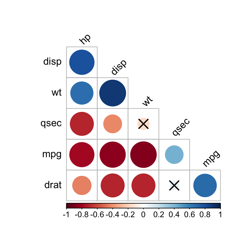
# Draw correlogram using R base plot
#::::::::::::::::::::::::::::::::::::::::::::::::::::::::::
cor.mat %>%
cor_reorder() %>%
pull_lower_triangle() %>%
cor_plot()