使用dplyr进行数据处理
王诗翔 · 2018-03-21
该部分学习内容来自《R for Data Science》。
在对数据进行可视化之前我们往往需要进行数据转换以得到可视化所需要的数据内容与格式。这里我们使用dplyr包操作2013年纽约市的航班起飞数据集(2013)。
准备
这部分我们聚焦于如何使用dplyr包,除ggplot2的另一个tidyverse核心成员。我们将使用nyclights13数据包解释关键的概念并使用ggplot2帮助理解数据。
# 导入包
library(nycflights13) # 请确保在使用前已经安装好这些包
library(tidyverse)
#> ── Attaching packages ──────────────────────────────────────────────────────────── tidyverse 1.3.0 ──
#> ✓ ggplot2 3.3.2     ✓ purrr   0.3.4
#> ✓ tibble  3.0.3     ✓ dplyr   1.0.0
#> ✓ tidyr   1.1.0     ✓ stringr 1.4.0
#> ✓ readr   1.3.1     ✓ forcats 0.5.0
#> ── Conflicts ─────────────────────────────────────────────────────────────── tidyverse_conflicts() ──
#> x dplyr::filter() masks stats::filter()
#> x dplyr::lag() masks stats::lag()注意一下你导入tidyverse包时给出的冲突信息(Conflicts),它告诉你dplyr覆盖了R基础包中的函数。如果你想要在载入tidyverse包后仍然使用这些函数,你需要使用函数的全名stats::filter()和stats::lag()进行调用。
nycflights13
我们将使用nycflights13::flights来探索dplyr包基本的数据操作动词。该数据集包含2013年336,776次航班起飞数据,来自美国交通统计局。
flights
#> # A tibble: 336,776 x 19
#>     year month   day dep_time sched_dep_time dep_delay arr_time sched_arr_time
#>    <int> <int> <int>    <int>          <int>     <dbl>    <int>          <int>
#>  1  2013     1     1      517            515         2      830            819
#>  2  2013     1     1      533            529         4      850            830
#>  3  2013     1     1      542            540         2      923            850
#>  4  2013     1     1      544            545        -1     1004           1022
#>  5  2013     1     1      554            600        -6      812            837
#>  6  2013     1     1      554            558        -4      740            728
#>  7  2013     1     1      555            600        -5      913            854
#>  8  2013     1     1      557            600        -3      709            723
#>  9  2013     1     1      557            600        -3      838            846
#> 10  2013     1     1      558            600        -2      753            745
#> # … with 336,766 more rows, and 11 more variables: arr_delay <dbl>,
#> #   carrier <chr>, flight <int>, tailnum <chr>, origin <chr>, dest <chr>,
#> # air_time <dbl>, distance <dbl>, hour <dbl>, minute <dbl>, time_hour <dttm>与基本包显示的普通数据集输出不同,这里适配地显示了在一个屏幕前几行和所有的列(我们可以使用View(flights)在Rstudio中查看数据集的所有信息。输出显示不同的原因是这个数据集是一个Tibble。Tibbles都是数据框data.frame,但经过改良以便于更好(在tidyverse生态中)工作。现在我们不必纠结于这些差异,在后续内容中我们会进行学习。
你可能已经注意到每个列名下面有三到四个字母的缩写。它们描述了每个变量的类型:
int代表整数dbl代表浮点数或者实数chr代表字符向量或者字符串dttm代表日期-时间
还有其他三种数据类型在本部分不会使用到,但后续我们会接触:
lgl代表逻辑向量,只含TRUE和FALSEfctr代表因子,R用它来代表含固定可能值的分类变量date代表日期
dplyr基础
这部分我们学习5个关键的dplyr函数,它可以让我们解决遇到的大部分数据操作问题:
- 根据值选择观察(记录),
filter() - 对行重新排序,
arrange() - 根据名字选择变量,
select() - 根据已知的变量创建新的变量,
mutate() - 将许多值塌缩为单个描述性汇总,
summarize()
这些函数都可以通过group_by()衔接起来,该函数改变上述每个函数的作用域,从操作整个数据集到按组与组操作。这六个函数提供了数据操作语言的动词。
所有的动词工作都非常相似:
- 第一个参数都是数据框
- 随后的参数描述了使用变量名(不加引号)对数据框做什么
- 结果是一个新的数据框
这些属性一起便利地将多个简单步骤串联起来得到一个复杂的操作(结果)。让我们实际来看看这些动词是怎么工作的。
使用filter()过滤行
filter()允许我们根据观测值来对数据集取子集。第一个参数是数据框的名字,第二和随后的参数是用于过滤数据框的表达式。
比如,我们可以选择所有一月一号的航班:
filter(flights, month == 1, day == 1)
#> # A tibble: 842 x 19
#>     year month   day dep_time sched_dep_time dep_delay arr_time sched_arr_time
#>    <int> <int> <int>    <int>          <int>     <dbl>    <int>          <int>
#>  1  2013     1     1      517            515         2      830            819
#>  2  2013     1     1      533            529         4      850            830
#>  3  2013     1     1      542            540         2      923            850
#>  4  2013     1     1      544            545        -1     1004           1022
#>  5  2013     1     1      554            600        -6      812            837
#>  6  2013     1     1      554            558        -4      740            728
#>  7  2013     1     1      555            600        -5      913            854
#>  8  2013     1     1      557            600        -3      709            723
#>  9  2013     1     1      557            600        -3      838            846
#> 10  2013     1     1      558            600        -2      753            745
#> # … with 832 more rows, and 11 more variables: arr_delay <dbl>, carrier <chr>,
#> #   flight <int>, tailnum <chr>, origin <chr>, dest <chr>, air_time <dbl>,
#> # distance <dbl>, hour <dbl>, minute <dbl>, time_hour <dttm>这一行代码dplyr执行了过滤操作并返回了一个新的数据框。dplyr从不修改输入数据,所以如果你想要保存数据,必须使用<-进行赋值:
jan1 <- filter(flights, month == 1, day == 1)R要么输出结果,要么将结果保存到一个变量。如果我们想要同时做到这一点,你可以把赋值放在括号里:
(dec25 <- filter(flights, month == 12, day == 25))
#> # A tibble: 719 x 19
#>     year month   day dep_time sched_dep_time dep_delay arr_time sched_arr_time
#>    <int> <int> <int>    <int>          <int>     <dbl>    <int>          <int>
#>  1  2013    12    25      456            500        -4      649            651
#>  2  2013    12    25      524            515         9      805            814
#>  3  2013    12    25      542            540         2      832            850
#>  4  2013    12    25      546            550        -4     1022           1027
#>  5  2013    12    25      556            600        -4      730            745
#>  6  2013    12    25      557            600        -3      743            752
#>  7  2013    12    25      557            600        -3      818            831
#>  8  2013    12    25      559            600        -1      855            856
#>  9  2013    12    25      559            600        -1      849            855
#> 10  2013    12    25      600            600         0      850            846
#> # … with 709 more rows, and 11 more variables: arr_delay <dbl>, carrier <chr>,
#> #   flight <int>, tailnum <chr>, origin <chr>, dest <chr>, air_time <dbl>,
#> #   distance <dbl>, hour <dbl>, minute <dbl>, time_hour <dttm>
比较
想要有效地过滤,你必须知道怎么利用比较操作符来选择观测值。R提供了标准的比较符:>,>=,<=,!=和==。
如果你是初学R,一个常见的错误是用=而不是==来检测相等。如果这种情况发生了,你会收到报错信息:
filter(flights, month = 1)
#> Error: `month` (`month = 1`) must not be named, do you need `==`?另一个你在使用==时可能遭遇的常见问题是浮点数。下面的结果可能会让你惊掉大牙:
sqrt(2) ^ 2 == 2
#> [1] FALSE
1/49 * 49 == 1
#> [1] FALSE
逻辑操作符
&是与,|是或,!是非。
下面代码找到在十一月或十二月起飞的所有航班:
filter(flights, month == 11 | month == 12)
#> # A tibble: 55,403 x 19
#>     year month   day dep_time sched_dep_time dep_delay arr_time sched_arr_time
#>    <int> <int> <int>    <int>          <int>     <dbl>    <int>          <int>
#>  1  2013    11     1        5           2359         6      352            345
#>  2  2013    11     1       35           2250       105      123           2356
#>  3  2013    11     1      455            500        -5      641            651
#>  4  2013    11     1      539            545        -6      856            827
#>  5  2013    11     1      542            545        -3      831            855
#>  6  2013    11     1      549            600       -11      912            923
#>  7  2013    11     1      550            600       -10      705            659
#>  8  2013    11     1      554            600        -6      659            701
#>  9  2013    11     1      554            600        -6      826            827
#> 10  2013    11     1      554            600        -6      749            751
#> # … with 55,393 more rows, and 11 more variables: arr_delay <dbl>,
#> #   carrier <chr>, flight <int>, tailnum <chr>, origin <chr>, dest <chr>,
#> # air_time <dbl>, distance <dbl>, hour <dbl>, minute <dbl>, time_hour <dttm>注意,你不能写成filter(flights, month == 11 | 12),(虽然语义上讲的通)对于R而言,它会先计算11|12得到1,然后计算month == 1,这就不是我们需要的了!
解决这种问题的一种有用简写为x %in% y。这将选择符合x属于y的行(x是y中的一个值)。我们可以用它重写前面的代码:
nov_dec <- filter(flights, month %in% c(11, 12))缺失值
NA代表未知值或者称为缺失值,它是能“传染”的,几乎任何涉及未知值的操作都会是一个未知值。
NA > 5
#> [1] NA
10 == NA
#> [1] NA
NA + 10
#> [1] NA
NA / 2
#> [1] NA
最让人困惑的结果是这个:
NA == NA
#> [1] NA最简单理解为什么这是TRUE的方式是带入一点语境:
# 把x看作小明的年龄,我们不知道他多大
x <- NA

# 把y看作小红的年龄,我们不知道她多大
y <- NA

# 小明和小红一样大吗?
x == y
#> [1] NA

# 我们不知道如果你想确定一个值是不是缺失了,使用is.na():
is.na(x)
#> [1] TRUEfilter()仅仅会包含条件是TRUE的行,把是FALSE或者NA的行排除。如果你想要保留缺失值,你可以显式地指定:
df <- tibble(x = c(1, NA, 3))
filter(df, x > 1)
#> # A tibble: 1 x 1
#>       x
#>   <dbl>
#> 1     3
filter(df, is.na(x) | x > 1)
#> # A tibble: 2 x 1
#>       x
#>   <dbl>
#> 1    NA
#> 2     3
练习
- 寻找满足以下条件的所有航班:
- 有一次大于等于2小时的航班抵达延误
- 飞去Houston(IAH或者HOU)
- 航空公司为United,American或者Delta (应当缩写是UA和DL)
- 在夏天起飞(July,August和September)
- 抵达延误超过两小时,但起飞时间正常
- 起飞时间在午夜到6.a.m之间(包含)
- 另一个有用的dplyr过滤助手是
between()函数。它是做什么的?你可以使用它简化用于解决前面问题的代码吗? - 有多少航班有一个缺失的
dep_time?其他缺失的变量有哪些?这些行表示什么呢? - 为什么
NA ^ 0不是缺失值?为什么NA | TRUE不是缺失值?为什么FALSE & NA不是缺失值?你可以弄懂它们的基本原理吗?
# 1
# 有一次大于等于2小时的航班抵达延误?
nrow(filter(flights, arr_delay >= 120))
#> [1] 10200
# 有很多抵达延误超过两小时的

# 飞去Houston(IAH或者HOU)?
nrow(filter(flights, dest %in% c("IAH", "HOU")))
#> [1] 9313
# 或者
nrow(filter(flights, dest == "IAH" | dest == "HOU"))
#> [1] 9313

# 航空公司为United,American或者Delta (应当缩写是UA和DL)
nrow(filter(flights, carrier %in% c("UA", "DL")))
#> [1] 106775

# 在夏天起飞(July,August和September)
nrow(filter(flights, month >=7 & month <=9))
#> [1] 86326

# 抵达延误超过两小时,但起飞时间正常
nrow(filter(flights, dep_delay == 0, arr_delay >= 120))
#> [1] 3

# 起飞时间在午夜到6.a.m之间(包含)
nrow(filter(flights, hour >= 0 & hour <= 6))
#> [1] 27905

# 2
# 先查看between()函数的用法
# help(between)
# 发现它可以用来替换left <= x & x <= right 这种情况
# 所以简化前面的结果就比较简单了
# 举个例子,比如查7到9月的航班
nrow(filter(flights, between(month, 7, 9)))
#> [1] 86326

# 3
nrow(filter(flights, is.na(dep_time)))
#> [1] 8255
# 所以有8000+航班缺起飞时间咯
# 接着看其他变量有缺失值没有
nrow(filter(flights, is.na(arr_time)))
#> [1] 8713
nrow(filter(flights, is.na(arr_time) & is.na(dep_time)))
#> [1] 8255
# 有8255次起飞与降落时间都未知!!
# 我猜测可能是航班取消了吧
# 你可以谈谈你的看法,进行更多探索,在下方留。

# 4
NA ^ 0
#> [1] 1
NA | TRUE
#> [1] TRUE
FALSE | NA
#> [1] NA
NA * 0
#> [1] NA

# 就我所见,应该用类型强制转换来解释这个问题
# 在解释性编程语言(R,Python)中,当操作涉及多个数据类型时
# 语言本身会按照特定的规则进行转换。具体网上搜索。
使用arrange()排列行
arrange()函数工作原理和filter()相似,但它不是选择行,而是改变行的顺序。它使用一个数据框和一系列有序的列变量(或者更复杂的表达式)作为输入。如果你提供了超过一个列名,其他列对应着进行排序。
arrange(flights, year, month, day)
#> # A tibble: 336,776 x 19
#>     year month   day dep_time sched_dep_time dep_delay arr_time sched_arr_time
#>    <int> <int> <int>    <int>          <int>     <dbl>    <int>          <int>
#>  1  2013     1     1      517            515         2      830            819
#>  2  2013     1     1      533            529         4      850            830
#>  3  2013     1     1      542            540         2      923            850
#>  4  2013     1     1      544            545        -1     1004           1022
#>  5  2013     1     1      554            600        -6      812            837
#>  6  2013     1     1      554            558        -4      740            728
#>  7  2013     1     1      555            600        -5      913            854
#>  8  2013     1     1      557            600        -3      709            723
#>  9  2013     1     1      557            600        -3      838            846
#> 10  2013     1     1      558            600        -2      753            745
#> # … with 336,766 more rows, and 11 more variables: arr_delay <dbl>,
#> #   carrier <chr>, flight <int>, tailnum <chr>, origin <chr>, dest <chr>,
#> # air_time <dbl>, distance <dbl>, hour <dbl>, minute <dbl>, time_hour <dttm>使用desc()可以以逆序(降序)的方式排列:
arrange(flights, desc(arr_delay))
#> # A tibble: 336,776 x 19
#>     year month   day dep_time sched_dep_time dep_delay arr_time sched_arr_time
#>    <int> <int> <int>    <int>          <int>     <dbl>    <int>          <int>
#>  1  2013     1     9      641            900      1301     1242           1530
#>  2  2013     6    15     1432           1935      1137     1607           2120
#>  3  2013     1    10     1121           1635      1126     1239           1810
#>  4  2013     9    20     1139           1845      1014     1457           2210
#>  5  2013     7    22      845           1600      1005     1044           1815
#>  6  2013     4    10     1100           1900       960     1342           2211
#>  7  2013     3    17     2321            810       911      135           1020
#>  8  2013     7    22     2257            759       898      121           1026
#>  9  2013    12     5      756           1700       896     1058           2020
#> 10  2013     5     3     1133           2055       878     1250           2215
#> # … with 336,766 more rows, and 11 more variables: arr_delay <dbl>,
#> #   carrier <chr>, flight <int>, tailnum <chr>, origin <chr>, dest <chr>,
#> #   air_time <dbl>, distance <dbl>, hour <dbl>, minute <dbl>, time_hour <dttm>
缺失值会排到最后面:
df <- tibble(x = c(5, 2, NA))
arrange(df, x)
#> # A tibble: 3 x 1
#>       x
#>   <dbl>
#> 1     2
#> 2     5
#> 3    NA
arrange(df, desc(x))
#> # A tibble: 3 x 1
#>       x
#>   <dbl>
#> 1     5
#> 2     2
#> 3    NA
练习
- 你怎么将所有的缺失值都排到最前面?(提示:使用
is.na()) - 给
flights排序找到延时最多的航班;找到其中离开最早的。 - 给
flights排序找到最快的航班。 - 哪一个航班时间最长?哪一个最短?
# 1
arrange(df, desc(is.na(x)))
#> # A tibble: 3 x 1
#>       x
#>   <dbl>
#> 1    NA
#> 2     5
#> 3     2
# 2
# 迟到最久
arrange(flights, desc(arr_delay))
#> # A tibble: 336,776 x 19
#>     year month   day dep_time sched_dep_time dep_delay arr_time sched_arr_time
#>    <int> <int> <int>    <int>          <int>     <dbl>    <int>          <int>
#>  1  2013     1     9      641            900      1301     1242           1530
#>  2  2013     6    15     1432           1935      1137     1607           2120
#>  3  2013     1    10     1121           1635      1126     1239           1810
#>  4  2013     9    20     1139           1845      1014     1457           2210
#>  5  2013     7    22      845           1600      1005     1044           1815
#>  6  2013     4    10     1100           1900       960     1342           2211
#>  7  2013     3    17     2321            810       911      135           1020
#>  8  2013     7    22     2257            759       898      121           1026
#>  9  2013    12     5      756           1700       896     1058           2020
#> 10  2013     5     3     1133           2055       878     1250           2215
#> # … with 336,766 more rows, and 11 more variables: arr_delay <dbl>,
#> #   carrier <chr>, flight <int>, tailnum <chr>, origin <chr>, dest <chr>,
#> #   air_time <dbl>, distance <dbl>, hour <dbl>, minute <dbl>, time_hour <dttm>
# 出发最早
arrange(flights, dep_delay)
#> # A tibble: 336,776 x 19
#>     year month   day dep_time sched_dep_time dep_delay arr_time sched_arr_time
#>    <int> <int> <int>    <int>          <int>     <dbl>    <int>          <int>
#>  1  2013    12     7     2040           2123       -43       40           2352
#>  2  2013     2     3     2022           2055       -33     2240           2338
#>  3  2013    11    10     1408           1440       -32     1549           1559
#>  4  2013     1    11     1900           1930       -30     2233           2243
#>  5  2013     1    29     1703           1730       -27     1947           1957
#>  6  2013     8     9      729            755       -26     1002            955
#>  7  2013    10    23     1907           1932       -25     2143           2143
#>  8  2013     3    30     2030           2055       -25     2213           2250
#>  9  2013     3     2     1431           1455       -24     1601           1631
#> 10  2013     5     5      934            958       -24     1225           1309
#> # … with 336,766 more rows, and 11 more variables: arr_delay <dbl>,
#> #   carrier <chr>, flight <int>, tailnum <chr>, origin <chr>, dest <chr>,
#> #   air_time <dbl>, distance <dbl>, hour <dbl>, minute <dbl>, time_hour <dttm>

# 3
# 最快的航班排序
arrange(flights, air_time)
#> # A tibble: 336,776 x 19
#>     year month   day dep_time sched_dep_time dep_delay arr_time sched_arr_time
#>    <int> <int> <int>    <int>          <int>     <dbl>    <int>          <int>
#>  1  2013     1    16     1355           1315        40     1442           1411
#>  2  2013     4    13      537            527        10      622            628
#>  3  2013    12     6      922            851        31     1021            954
#>  4  2013     2     3     2153           2129        24     2247           2224
#>  5  2013     2     5     1303           1315       -12     1342           1411
#>  6  2013     2    12     2123           2130        -7     2211           2225
#>  7  2013     3     2     1450           1500       -10     1547           1608
#>  8  2013     3     8     2026           1935        51     2131           2056
#>  9  2013     3    18     1456           1329        87     1533           1426
#> 10  2013     3    19     2226           2145        41     2305           2246
#> # … with 336,766 more rows, and 11 more variables: arr_delay <dbl>,
#> #   carrier <chr>, flight <int>, tailnum <chr>, origin <chr>, dest <chr>,
#> #   air_time <dbl>, distance <dbl>, hour <dbl>, minute <dbl>, time_hour <dttm>

# 4
# 最长的航班
arrange(flights, desc(air_time))[1,]
#> # A tibble: 1 x 19
#>    year month   day dep_time sched_dep_time dep_delay arr_time sched_arr_time
#>   <int> <int> <int>    <int>          <int>     <dbl>    <int>          <int>
#> 1  2013     3    17     1337           1335         2     1937           1836
#> # … with 11 more variables: arr_delay <dbl>, carrier <chr>, flight <int>,
#> #   tailnum <chr>, origin <chr>, dest <chr>, air_time <dbl>, distance <dbl>,
#> #   hour <dbl>, minute <dbl>, time_hour <dttm>
# 最快的航班
arrange(flights, air_time)[1,]
#> # A tibble: 1 x 19
#>    year month   day dep_time sched_dep_time dep_delay arr_time sched_arr_time
#>   <int> <int> <int>    <int>          <int>     <dbl>    <int>          <int>
#> 1  2013     1    16     1355           1315        40     1442           1411
#> # … with 11 more variables: arr_delay <dbl>, carrier <chr>, flight <int>,
#> #   tailnum <chr>, origin <chr>, dest <chr>, air_time <dbl>, distance <dbl>,
#> #   hour <dbl>, minute <dbl>, time_hour <dttm>
使用select()选择列
一般我们分析的原始数据集有非常多的变量(列),第一个我们要解决的问题就是缩小范围找到我们需要的数据(变量)。select()允许我们快速通过变量名对数据集取子集。
# 根据名字选择列
select(flights, year, month, day)
#> # A tibble: 336,776 x 3
#>     year month   day
#>    <int> <int> <int>
#>  1  2013     1     1
#>  2  2013     1     1
#>  3  2013     1     1
#>  4  2013     1     1
#>  5  2013     1     1
#>  6  2013     1     1
#>  7  2013     1     1
#>  8  2013     1     1
#>  9  2013     1     1
#> 10  2013     1     1
#> # … with 336,766 more rows

# 选择year到day之间(包含本身)的所有列
select(flights, year:day)
#> # A tibble: 336,776 x 3
#>     year month   day
#>    <int> <int> <int>
#>  1  2013     1     1
#>  2  2013     1     1
#>  3  2013     1     1
#>  4  2013     1     1
#>  5  2013     1     1
#>  6  2013     1     1
#>  7  2013     1     1
#>  8  2013     1     1
#>  9  2013     1     1
#> 10  2013     1     1
#> # … with 336,766 more rows

# 选择那么除year到day的所有列
select(flights, -(year:day))
#> # A tibble: 336,776 x 16
#>    dep_time sched_dep_time dep_delay arr_time sched_arr_time arr_delay carrier
#>       <int>          <int>     <dbl>    <int>          <int>     <dbl> <chr>
#>  1      517            515         2      830            819        11 UA
#>  2      533            529         4      850            830        20 UA
#>  3      542            540         2      923            850        33 AA
#>  4      544            545        -1     1004           1022       -18 B6
#>  5      554            600        -6      812            837       -25 DL
#>  6      554            558        -4      740            728        12 UA
#>  7      555            600        -5      913            854        19 B6
#>  8      557            600        -3      709            723       -14 EV
#>  9      557            600        -3      838            846        -8 B6
#> 10      558            600        -2      753            745         8 AA
#> # … with 336,766 more rows, and 9 more variables: flight <int>, tailnum <chr>,
#> #   origin <chr>, dest <chr>, air_time <dbl>, distance <dbl>, hour <dbl>,
#> # minute <dbl>, time_hour <dttm>有很多帮助函数可以使用在select()函数中:
starts_with("abc")匹配以“abc”开头的名字。ends_with("xyz")匹配以“xyz”结尾的名字。contains("ijk")匹配包含“ijk”的名字。matches("(.)\\1")选择符合正则表达式的变量。这里是任意包含有重复字符的变量。num_range("x", 1:3)匹配x1,x2,x3。
运行?select查看更多详情。
select()也可以用来重命名变量,但很少使用到,因为它会将所有未显示指定的变量删除掉。我们可以使用它的变体函数rename()来给变量重新命名:
rename(flights, tail_num = tailnum)
#> # A tibble: 336,776 x 19
#>     year month   day dep_time sched_dep_time dep_delay arr_time sched_arr_time
#>    <int> <int> <int>    <int>          <int>     <dbl>    <int>          <int>
#>  1  2013     1     1      517            515         2      830            819
#>  2  2013     1     1      533            529         4      850            830
#>  3  2013     1     1      542            540         2      923            850
#>  4  2013     1     1      544            545        -1     1004           1022
#>  5  2013     1     1      554            600        -6      812            837
#>  6  2013     1     1      554            558        -4      740            728
#>  7  2013     1     1      555            600        -5      913            854
#>  8  2013     1     1      557            600        -3      709            723
#>  9  2013     1     1      557            600        -3      838            846
#> 10  2013     1     1      558            600        -2      753            745
#> # … with 336,766 more rows, and 11 more variables: arr_delay <dbl>,
#> #   carrier <chr>, flight <int>, tail_num <chr>, origin <chr>, dest <chr>,
#> # air_time <dbl>, distance <dbl>, hour <dbl>, minute <dbl>, time_hour <dttm>select()的另外一个操作是与everything()帮助函数联合使用。当你有一大堆变量你想要移动到数据框开始(最左侧)时非常有用。
select(flights, time_hour, air_time, everything())
#> # A tibble: 336,776 x 19
#>    time_hour           air_time  year month   day dep_time sched_dep_time
#>    <dttm>                 <dbl> <int> <int> <int>    <int>          <int>
#>  1 2013-01-01 05:00:00      227  2013     1     1      517            515
#>  2 2013-01-01 05:00:00      227  2013     1     1      533            529
#>  3 2013-01-01 05:00:00      160  2013     1     1      542            540
#>  4 2013-01-01 05:00:00      183  2013     1     1      544            545
#>  5 2013-01-01 06:00:00      116  2013     1     1      554            600
#>  6 2013-01-01 05:00:00      150  2013     1     1      554            558
#>  7 2013-01-01 06:00:00      158  2013     1     1      555            600
#>  8 2013-01-01 06:00:00       53  2013     1     1      557            600
#>  9 2013-01-01 06:00:00      140  2013     1     1      557            600
#> 10 2013-01-01 06:00:00      138  2013     1     1      558            600
#> # … with 336,766 more rows, and 12 more variables: dep_delay <dbl>,
#> #   arr_time <int>, sched_arr_time <int>, arr_delay <dbl>, carrier <chr>,
#> #   flight <int>, tailnum <chr>, origin <chr>, dest <chr>, distance <dbl>,
#> #   hour <dbl>, minute <dbl>
练习
- 尽量用更多的方式从
flights中选择dep_time,dep_delay,arr_time和arr_delay。 - 如果你多次包含同一变量名在
select()函数里会发生什么呢? one_of()函数是用来做什么的?为什么它与下面这个向量结合使用会非常有用?
    var <- c(
    "year", "month", "day", "dep_delay", "arr_delay"
)- 下面代码的运行结果会让你吃惊吗?这个
select的帮助函数默认是怎样处理这种情况的呢?你怎样改变默认的情况?
# 1
# 基本select用法,使用:,使用-去除其他的,使用%in%等等

# 2
select(flights, year, year)
#> # A tibble: 336,776 x 1
#>     year
#>    <int>
#>  1  2013
#>  2  2013
#>  3  2013
#>  4  2013
#>  5  2013
#>  6  2013
#>  7  2013
#>  8  2013
#>  9  2013
#> 10  2013
#> # … with 336,766 more rows
# 只会选择一次

# 3
# `one_of()`函数
vars <- c("year", "month", "day", "dep_delay", "arr_delay")
select(flights,  one_of(vars))
#> # A tibble: 336,776 x 5
#>     year month   day dep_delay arr_delay
#>    <int> <int> <int>     <dbl>     <dbl>
#>  1  2013     1     1         2        11
#>  2  2013     1     1         4        20
#>  3  2013     1     1         2        33
#>  4  2013     1     1        -1       -18
#>  5  2013     1     1        -6       -25
#>  6  2013     1     1        -4        12
#>  7  2013     1     1        -5        19
#>  8  2013     1     1        -3       -14
#>  9  2013     1     1        -3        -8
#> 10  2013     1     1        -2         8
#> # … with 336,766 more rows
# 这种用法可以有效地按数据情况进行选择而不会报错

# 4
select(flights, contains("TIME"))
#> # A tibble: 336,776 x 6
#>    dep_time sched_dep_time arr_time sched_arr_time air_time time_hour
#>       <int>          <int>    <int>          <int>    <dbl> <dttm>
#>  1      517            515      830            819      227 2013-01-01 05:00:00
#>  2      533            529      850            830      227 2013-01-01 05:00:00
#>  3      542            540      923            850      160 2013-01-01 05:00:00
#>  4      544            545     1004           1022      183 2013-01-01 05:00:00
#>  5      554            600      812            837      116 2013-01-01 06:00:00
#>  6      554            558      740            728      150 2013-01-01 05:00:00
#>  7      555            600      913            854      158 2013-01-01 06:00:00
#>  8      557            600      709            723       53 2013-01-01 06:00:00
#>  9      557            600      838            846      140 2013-01-01 06:00:00
#> 10      558            600      753            745      138 2013-01-01 06:00:00
#> # … with 336,766 more rows
# 看来函数没有找到`TIME`列,所以输出了所有列
# 想要更改,我们要查看该函数的参数
args(contains)
#> function (match, ignore.case = TRUE, vars = NULL)
#> NULL
使用mutate()添加新变量
除了选择已存在的列,另一个常见的操作是添加新的列。这就是mutate()函数的工作了。
mutate()函数通常将新增变量放在数据集的最后面。为了看到新生成的变量,我们使用一个小的数据集。
flights_sml <- select(flights,
                      year:day,
                      ends_with("delay"),
                      distance,
                      air_time)

mutate(flights_sml,
       gain = arr_delay - dep_delay,
       speed = distance / air_time * 60)
#> # A tibble: 336,776 x 9
#>     year month   day dep_delay arr_delay distance air_time  gain speed
#>    <int> <int> <int>     <dbl>     <dbl>    <dbl>    <dbl> <dbl> <dbl>
#>  1  2013     1     1         2        11     1400      227     9  370.
#>  2  2013     1     1         4        20     1416      227    16  374.
#>  3  2013     1     1         2        33     1089      160    31  408.
#>  4  2013     1     1        -1       -18     1576      183   -17  517.
#>  5  2013     1     1        -6       -25      762      116   -19  394.
#>  6  2013     1     1        -4        12      719      150    16  288.
#>  7  2013     1     1        -5        19     1065      158    24  404.
#>  8  2013     1     1        -3       -14      229       53   -11  259.
#>  9  2013     1     1        -3        -8      944      140    -5  405.
#> 10  2013     1     1        -2         8      733      138    10  319.
#> # … with 336,766 more rows

mutate(flights_sml,
       gain = arr_delay - dep_delay,
       hours = air_time / 60,
       gain_per_hour = gain / hours)
#> # A tibble: 336,776 x 10
#>     year month   day dep_delay arr_delay distance air_time  gain hours
#>    <int> <int> <int>     <dbl>     <dbl>    <dbl>    <dbl> <dbl> <dbl>
#>  1  2013     1     1         2        11     1400      227     9 3.78
#>  2  2013     1     1         4        20     1416      227    16 3.78
#>  3  2013     1     1         2        33     1089      160    31 2.67
#>  4  2013     1     1        -1       -18     1576      183   -17 3.05
#>  5  2013     1     1        -6       -25      762      116   -19 1.93
#>  6  2013     1     1        -4        12      719      150    16 2.5
#>  7  2013     1     1        -5        19     1065      158    24 2.63
#>  8  2013     1     1        -3       -14      229       53   -11 0.883
#>  9  2013     1     1        -3        -8      944      140    -5 2.33
#> 10  2013     1     1        -2         8      733      138    10 2.3
#> # … with 336,766 more rows, and 1 more variable: gain_per_hour <dbl>如果你仅仅想要保存新的变量,使用transmute():
transmute(flights,
          gain = arr_delay - dep_delay,
          hours = air_time / 60,
          gain_per_hour = gain / hours)
#> # A tibble: 336,776 x 3
#>     gain hours gain_per_hour
#>    <dbl> <dbl>         <dbl>
#>  1     9 3.78           2.38
#>  2    16 3.78           4.23
#>  3    31 2.67          11.6
#>  4   -17 3.05          -5.57
#>  5   -19 1.93          -9.83
#>  6    16 2.5            6.4
#>  7    24 2.63           9.11
#>  8   -11 0.883        -12.5
#>  9    -5 2.33          -2.14
#> 10    10 2.3            4.35
#> # … with 336,766 more rows
有用的创造函数
有很多函数可以结合mutate()一起使用来创造新的变量。这些函数的一个关键属性就是向量化的:它必须使用一组向量值作为输入,然后返回相同长度的数值作为输出。我们没有办法将所有的函数都列举出来,这里选择一些被频繁使用的函数。
算术操作符
- 算术操作符本质都是向量化的函数,遵循“循环补齐”的规则。如果一个参数比另一个参数短,它会自动扩展为后者同样的长度。比如
air_time / 60,hours * 60等等。
模运算(%/%和%%)
%/%整除和%%取余。
对数
log(),log2()和log10()
位移量/偏移量
lead()和lag()允许你前移或后移变量的值。
(x <- 1:10)
#>  [1]  1  2  3  4  5  6  7  8  9 10
lag(x)
#>  [1] NA  1  2  3  4  5  6  7  8  9
lead(x)
#>  [1]  2  3  4  5  6  7  8  9 10 NA
累积计算
- R提供了累积和、累积积、和累积最小值、和累积最大值:
cumsum(),cumprod(),cummin(),cummax()。dplyr提供勒cummean()用于计算累积平均值。如果你想要进行滚动累积计算,可以尝试下RcppRoll包。
x
#>  [1]  1  2  3  4  5  6  7  8  9 10
cumsum(x)
#>  [1]  1  3  6 10 15 21 28 36 45 55
cummean(x)
#>  [1] 1.00 1.00 1.33 1.75 2.20 2.67 3.14 3.62 4.11 4.60
逻辑比较
<,<=,>,>=,!=
排序rank
- 存在很多rank函数,但我们从
min_rank()的使用开始,它可以实现最常见的rank(例如第一、第二、第三、第四),使用desc()进行辅助可以给最大值最小的rank。
y <- c(1,2,2,NA,3,4)
min_rank(y)
#> [1]  1  2  2 NA  4  5
min_rank(desc(y))
#> [1] 5 3 3 NA 2 1如果min_rank()解决不了你的需求,看看变种row_number()、dense_rank()、percent_rank()、cume_dist()和ntile(),查看他们的帮助页面获取使用方法。
row_number(y)
#> [1]  1  2  3 NA  4  5
dense_rank(y)
#> [1]  1  2  2 NA  3  4
percent_rank(y)
#> [1] 0.00 0.25 0.25   NA 0.75 1.00
cume_dist(y)
#> [1] 0.2 0.6 0.6  NA 0.8 1.0
使用summarize()计算汇总值
最后一个关键的动词是summarize(),它将一个数据框坍缩为单个行:
summarize(flights, delay = mean(dep_delay, na.rm = TRUE))
#> # A tibble: 1 x 1
#>   delay
#>   <dbl>
#> 1 12.6除非我们将summarize()与group_by()配对使用,不然summarize()显得没啥用。这个操作会将分析单元从整个数据集转到单个的组别。然后,当你使用dplyr动词对分组的数据框进行操作时,它会自动进行分组计算。比如,我们想要按日期分组,得到每个日期的平均延期:
by_day <- group_by(flights, year, month, day)
summarize(by_day, delay = mean(dep_delay, na.rm = TRUE))
#> `summarise()` regrouping output by 'year', 'month' (override with `.groups` argument)
#> # A tibble: 365 x 4
#> # Groups:   year, month [12]
#>     year month   day delay
#>    <int> <int> <int> <dbl>
#>  1  2013     1     1 11.5
#>  2  2013     1     2 13.9
#>  3  2013     1     3 11.0
#>  4  2013     1     4  8.95
#>  5  2013     1     5  5.73
#>  6  2013     1     6  7.15
#>  7  2013     1     7  5.42
#>  8  2013     1     8  2.55
#>  9  2013     1     9  2.28
#> 10  2013     1    10  2.84
#> # … with 355 more rowsgroup_by()与summarize()的联合使用是我们最常用的dplyr工具:进行分组汇总。在我们进一步学习之前,我们需要了解一个非常强大的思想:管道。
使用管道整合多个操作
想象你要探索每个位置距离和平均航班延迟的关系。使用你已经知道的dplyr知识,你可能会写出下面的代码:
by_dest <- group_by(flights, dest)
delay <- summarize(by_dest,
                   count = n(),
                   dist = mean(distance, na.rm = TRUE),
                   delay = mean(arr_delay, na.rm = TRUE) )
#> `summarise()` ungrouping output (override with `.groups` argument)
delay <- filter(delay, count > 20, dest != "HNL")
ggplot(data = delay, mapping = aes(x = dist, y = delay)) +
geom_point(aes(size=count), alpha = 1/3) +
geom_smooth(se = FALSE)
#> `geom_smooth()` using method = 'loess' and formula 'y ~ x'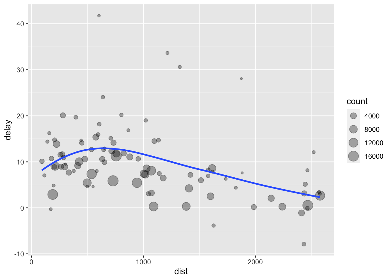
看起来在大概750英里之前,距离增大,延误时间也增加;随后减少。可能是航班长了之后,飞机更有能力在空中进行调整?
上述代码分三步进行了数据准备:
- 按目的地将航班分组
- 汇总计算距离、平均延时和航班数目
- 移除噪声点和Honolulu航班,它太远了。
这个代码写的有点令人沮丧,尽管我们不关心中间变量(临时变量),但我们却不得不创造这些中间变量存储结果数据框。命名是一件非常困难的事情,它会降低我们分析的速度。
另一种方式可以解决同样的问题,这就是管道pipe,%>:
delays <- flights %>%
    group_by(dest) %>%
    summarize(
        count = n(),
        dist = mean(distance, na.rm = TRUE),
        delay = mean(arr_delay, na.rm = TRUE)
    ) %>%
    filter(count > 20, dest != "HNL")
#> `summarise()` ungrouping output (override with `.groups` argument)这代码聚焦于转换,而不是什么被转换,这让代码更容易阅读。你可以将这段代码当作命令式的语句:分组、然后汇总,然后过滤。对%>%理解的一种好的方式就是将它发音为”然后“。
在后台,x %>% f(y)会变成f(x, y),x %>% f(y) %>% g(z)会变成g(f(x, y), z)等等如此。你可以使用管道——用一种从上到下,从左到右的的方式重写多个操作。从现在开始我们将会频繁地用到管道,因为它会提升代码的可读性,这些我们会在后续进行深入学习。
使用管道进行工作是属于tidyverse的一个重要标准。唯一的例外是ggplot2,它在管道开发之前就已经写好了。不幸的是,ggplot2的下一个版本ggvis会使用管道,但还没有发布。
缺失值
你可能会好奇我们先前使用的na.rm参数。如果我们不设置它会发生什么呢?
flights %>%
    group_by(dest) %>%
    summarize(
        count = n(),
        dist = mean(distance),
        delay = mean(arr_delay)
    ) %>%
    filter(count > 20, dest != "HNL")
#> `summarise()` ungrouping output (override with `.groups` argument)
#> # A tibble: 96 x 4
#>    dest  count  dist delay
#>    <chr> <int> <dbl> <dbl>
#>  1 ABQ     254 1826   4.38
#>  2 ACK     265  199  NA
#>  3 ALB     439  143  NA
#>  4 ATL   17215  757. NA
#>  5 AUS    2439 1514. NA
#>  6 AVL     275  584. NA
#>  7 BDL     443  116  NA
#>  8 BGR     375  378  NA
#>  9 BHM     297  866. NA
#> 10 BNA    6333  758. NA
#> # … with 86 more rows我们得到了一堆缺失值!如果输入不去除缺失值,结果必然是缺失值。幸运的是,所有的聚集函数都有na.rm参数,它可以在计算之前移除缺失值。
flights %>%
    group_by(year, month, day) %>%
    summarize(mean = mean(dep_delay, na.rm = TRUE))
#> `summarise()` regrouping output by 'year', 'month' (override with `.groups` argument)
#> # A tibble: 365 x 4
#> # Groups:   year, month [12]
#>     year month   day  mean
#>    <int> <int> <int> <dbl>
#>  1  2013     1     1 11.5
#>  2  2013     1     2 13.9
#>  3  2013     1     3 11.0
#>  4  2013     1     4  8.95
#>  5  2013     1     5  5.73
#>  6  2013     1     6  7.15
#>  7  2013     1     7  5.42
#>  8  2013     1     8  2.55
#>  9  2013     1     9  2.28
#> 10  2013     1    10  2.84
#> # … with 355 more rows
这个例子中,缺失值代表了取消的航班,所以我们解决这样问题的办法就是首先移除取消的航班。
not_cancelled <- flights %>%
    filter(!is.na(dep_delay), !is.na(arr_delay))

not_cancelled %>%
    group_by(year, month, day) %>%
    summarize(mean = mean(dep_delay))
#> `summarise()` regrouping output by 'year', 'month' (override with `.groups` argument)
#> # A tibble: 365 x 4
#> # Groups:   year, month [12]
#>     year month   day  mean
#>    <int> <int> <int> <dbl>
#>  1  2013     1     1 11.4
#>  2  2013     1     2 13.7
#>  3  2013     1     3 10.9
#>  4  2013     1     4  8.97
#>  5  2013     1     5  5.73
#>  6  2013     1     6  7.15
#>  7  2013     1     7  5.42
#>  8  2013     1     8  2.56
#>  9  2013     1     9  2.30
#> 10  2013     1    10  2.84
#> # … with 355 more rows
计数
无论什么时候你进行汇总,包含计数n()或者非缺失值计数sum(!is.na(x))总是一个好想法。这样你可以检查你下结论来源的数据数目。例如,让我们看下有最高平均延时的飞机(根据尾号识别):
delays <- not_cancelled %>%
    group_by(tailnum) %>%
    summarize(
        delay = mean(arr_delay)
    )
#> `summarise()` ungrouping output (override with `.groups` argument)

ggplot(data = delays, mapping = aes(x = delay)) +
    geom_freqpoly(binwidth = 10)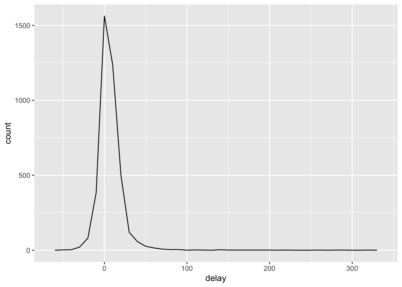
哇!居然有些飞机平均延时5个小时(300分钟)。
绘制平均延时下航班数目的散点图可以呈现更多的信息:
delays <- not_cancelled %>%
    group_by(tailnum) %>%
    summarize(
        delay = mean(arr_delay, na.rm = TRUE),
        n = n()
    )
#> `summarise()` ungrouping output (override with `.groups` argument)

ggplot(data = delays, mapping = aes(x = n, y = delay)) +
    geom_point(alpha = 1/10)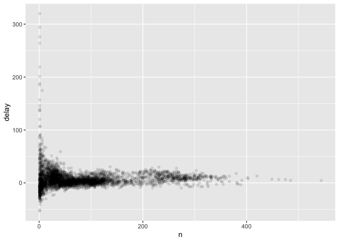
当航班数少时平均延时存在很大的变异,这并不奇怪。这个图的形状很有特征性:无论什么时候你按照组别绘制均值(或其他汇总量),你会看到变异会随着样本量的增加而减少。
当你看到这种类型图时,过滤掉有很少数目的组别是很有用的,可以看到数据更多的模式和更少的极端值。这正是下面代码做的事情,它同时展示了整合dplyr与ggplot2的一种手动方式。突然从%>%转换到+可能会感觉有点伤,但习惯了就会感觉很便利啦:
delays %>%
    filter(n > 25) %>%
    ggplot(mapping = aes(x = n, y = delay)) +
    geom_point(alpha = 1/10)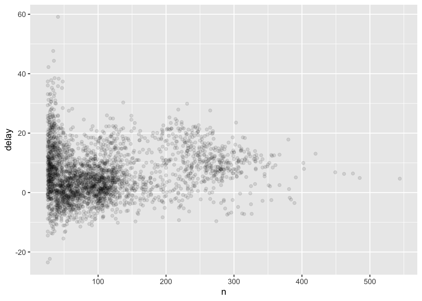
让我们看另一个例子:棒球运动中击球手的平均表现与上场击球次数的关系。这里我们使用来自Lahman包的数据计算每个选手平均成功率(击球平均得分数,击球数/尝试数)。
当我画出击球手技能(用成功率衡量)与击球的机会数关系时,你会看到两种模式:
- 数据点越多,变异越少
- 选手技能和击球机会成正相关关系。这是因为队伍可以控制谁可以上场,很显然他们都会选自己最棒的选手:
# 转换为tibble,看起来更舒服
batting <- as.tibble(Lahman::Batting)
#> Warning: `as.tibble()` is deprecated as of tibble 2.0.0.
#> Please use `as_tibble()` instead.
#> The signature and semantics have changed, see `?as_tibble`.
#> This warning is displayed once every 8 hours.
#> Call `lifecycle::last_warnings()` to see where this warning was generated.

batters <- batting %>%
    group_by(playerID) %>%
    summarize(
        ba = sum(H, na.rm = TRUE) / sum(AB, na.rm = TRUE),
        ab = sum(AB, na.rm = TRUE)
    )
#> `summarise()` ungrouping output (override with `.groups` argument)

batters %>%
    filter(ab > 100) %>%
    ggplot(mapping = aes(x = ab, y = ba)) +
    geom_point() +
    geom_smooth(se = FALSE)
#> `geom_smooth()` using method = 'gam' and formula 'y ~ s(x, bs = "cs")'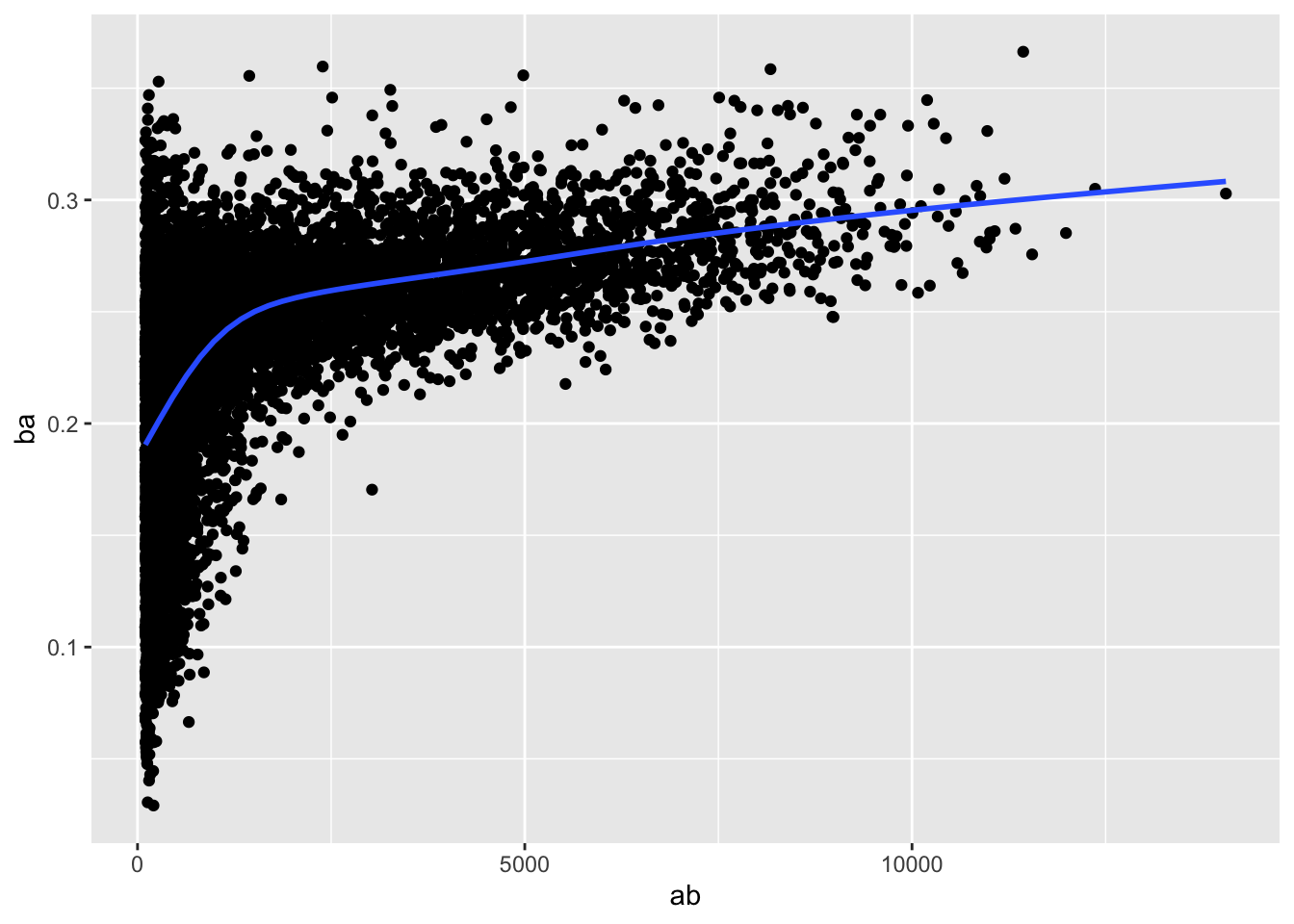
有用的汇总函数
仅仅使用均值、计数和求和这些函数就可以帮我做很多事情,但R提供了许多其他有用的汇总函数:
位置度量
- 我们已经使用过
mean()函数求取平均值(总和除以长度),median()函数也非常有用,它会找到中位数。
有时候整合聚集函数和逻辑操作符是非常有用的:
not_cancelled %>%
    group_by(year, month, day) %>%
    summarize(
        # 平均延时
        avg_delay1 = mean(arr_delay),
        # 平均正延时
        avg_delay2 = mean(arr_delay[arr_delay > 0])
    )
#> `summarise()` regrouping output by 'year', 'month' (override with `.groups` argument)
#> # A tibble: 365 x 5
#> # Groups:   year, month [12]
#>     year month   day avg_delay1 avg_delay2
#>    <int> <int> <int>      <dbl>      <dbl>
#>  1  2013     1     1     12.7         32.5
#>  2  2013     1     2     12.7         32.0
#>  3  2013     1     3      5.73        27.7
#>  4  2013     1     4     -1.93        28.3
#>  5  2013     1     5     -1.53        22.6
#>  6  2013     1     6      4.24        24.4
#>  7  2013     1     7     -4.95        27.8
#>  8  2013     1     8     -3.23        20.8
#>  9  2013     1     9     -0.264       25.6
#> 10  2013     1    10     -5.90        27.3
#> # … with 355 more rows分布度量sd(x),IQR(x),mad(x)
sd()计算均方差(也称为标准差或简写为sd),是分布的标准度量;IQR()计算四分位数极差;mad()计算中位绝对离差(存在离群点时,是更稳定的IQR值等价物)。
# 为何到某些目的地航班的距离比其他存在更多变异
not_cancelled %>%
    group_by(dest) %>%
    summarize(distance_sd = sd(distance)) %>%
    arrange(desc(distance_sd))
#> `summarise()` ungrouping output (override with `.groups` argument)
#> # A tibble: 104 x 2
#>    dest  distance_sd
#>    <chr>       <dbl>
#>  1 EGE         10.5
#>  2 SAN         10.4
#>  3 SFO         10.2
#>  4 HNL         10.0
#>  5 SEA          9.98
#>  6 LAS          9.91
#>  7 PDX          9.87
#>  8 PHX          9.86
#>  9 LAX          9.66
#> 10 IND          9.46
#> # … with 94 more rows
等级度量 min(x),quantile(x, 0.25),max(x)
分位数是中位数更通用化的一种形式。比如,quantile(x, 0.25)会找到x中刚好大于25%的值而小于7%的值的那个数。
# 每天第一班飞机和最后一般飞机是什么时候?
not_cancelled %>%
    group_by(year, month, day) %>%
    summarize(
        first = min(dep_time),
        last = max(dep_time)
    )
#> `summarise()` regrouping output by 'year', 'month' (override with `.groups` argument)
#> # A tibble: 365 x 5
#> # Groups:   year, month [12]
#>     year month   day first  last
#>    <int> <int> <int> <int> <int>
#>  1  2013     1     1   517  2356
#>  2  2013     1     2    42  2354
#>  3  2013     1     3    32  2349
#>  4  2013     1     4    25  2358
#>  5  2013     1     5    14  2357
#>  6  2013     1     6    16  2355
#>  7  2013     1     7    49  2359
#>  8  2013     1     8   454  2351
#>  9  2013     1     9     2  2252
#> 10  2013     1    10     3  2320
#> # … with 355 more rows
位置度量 first(x), nth(x, 2), last(x)
这些函数跟x[1],x[2],x[length(x)]工作相似,但是如果该位置不存在会返回一个默认值。例如,我们想找到每天起飞的第一班和最后一班飞机:
not_cancelled %>%
    group_by(year, month, day) %>%
    summarize(
        first_dep = first(dep_time),
        last_dep = last(dep_time)
    )
#> `summarise()` regrouping output by 'year', 'month' (override with `.groups` argument)
#> # A tibble: 365 x 5
#> # Groups:   year, month [12]
#>     year month   day first_dep last_dep
#>    <int> <int> <int>     <int>    <int>
#>  1  2013     1     1       517     2356
#>  2  2013     1     2        42     2354
#>  3  2013     1     3        32     2349
#>  4  2013     1     4        25     2358
#>  5  2013     1     5        14     2357
#>  6  2013     1     6        16     2355
#>  7  2013     1     7        49     2359
#>  8  2013     1     8       454     2351
#>  9  2013     1     9         2     2252
#> 10  2013     1    10         3     2320
#> # … with 355 more rows
这些函数可以与基于rank的函数互补:
not_cancelled %>%
    group_by(year, month, day) %>%
    mutate(r = min_rank(desc(dep_time))) %>%
    filter(r %in% range(r))
#> # A tibble: 770 x 20
#> # Groups:   year, month, day [365]
#>     year month   day dep_time sched_dep_time dep_delay arr_time sched_arr_time
#>    <int> <int> <int>    <int>          <int>     <dbl>    <int>          <int>
#>  1  2013     1     1      517            515         2      830            819
#>  2  2013     1     1     2356           2359        -3      425            437
#>  3  2013     1     2       42           2359        43      518            442
#>  4  2013     1     2     2354           2359        -5      413            437
#>  5  2013     1     3       32           2359        33      504            442
#>  6  2013     1     3     2349           2359       -10      434            445
#>  7  2013     1     4       25           2359        26      505            442
#>  8  2013     1     4     2358           2359        -1      429            437
#>  9  2013     1     4     2358           2359        -1      436            445
#> 10  2013     1     5       14           2359        15      503            445
#> # … with 760 more rows, and 12 more variables: arr_delay <dbl>, carrier <chr>,
#> #   flight <int>, tailnum <chr>, origin <chr>, dest <chr>, air_time <dbl>,
#> #   distance <dbl>, hour <dbl>, minute <dbl>, time_hour <dttm>, r <int>
计数
你已经见过了n()函数,它没有任何参数并返回当前组别的大小。为了对非缺失值计数,使用sum(!is.na(x))。要对唯一值进行计数,使用n_distinct():
# 哪个目的地有最多的carrier
not_cancelled %>%
    group_by(dest) %>%
    summarize(carriers = n_distinct(carrier)) %>%
    arrange(desc(carriers))
#> `summarise()` ungrouping output (override with `.groups` argument)
#> # A tibble: 104 x 2
#>    dest  carriers
#>    <chr>    <int>
#>  1 ATL          7
#>  2 BOS          7
#>  3 CLT          7
#>  4 ORD          7
#>  5 TPA          7
#>  6 AUS          6
#>  7 DCA          6
#>  8 DTW          6
#>  9 IAD          6
#> 10 MSP          6
#> # … with 94 more rows计数十分有用,如果你仅仅想要计数,dplyr提供了一个帮助函数:
not_cancelled %>%
    count(dest)
#> # A tibble: 104 x 2
#>    dest      n
#>    <chr> <int>
#>  1 ABQ     254
#>  2 ACK     264
#>  3 ALB     418
#>  4 ANC       8
#>  5 ATL   16837
#>  6 AUS    2411
#>  7 AVL     261
#>  8 BDL     412
#>  9 BGR     358
#> 10 BHM     269
#> # … with 94 more rows
你可以选择性提供一个权重变量。比如,你想用它计数(求和)一个飞机飞行的总里程:
not_cancelled %>%
    count(tailnum, wt = distance)
#> # A tibble: 4,037 x 2
#>    tailnum      n
#>    <chr>    <dbl>
#>  1 D942DN    3418
#>  2 N0EGMQ  239143
#>  3 N10156  109664
#>  4 N102UW   25722
#>  5 N103US   24619
#>  6 N104UW   24616
#>  7 N10575  139903
#>  8 N105UW   23618
#>  9 N107US   21677
#> 10 N108UW   32070
#> # … with 4,027 more rows
计数与逻辑值比例 sum(x > 10), mean(y == 0)
当与数值函数使用时,TRUE被转换为1,FALSE被转换为0。这让sum()与mean()变得非常有用,sum(x)可以计算x中TRUE的数目,mean()可以计算比例:
# 多少航班在5点前离开
not_cancelled %>%
    group_by(year, month, day) %>%
    summarize(n_early = sum(dep_time < 500))
#> `summarise()` regrouping output by 'year', 'month' (override with `.groups` argument)
#> # A tibble: 365 x 4
#> # Groups:   year, month [12]
#>     year month   day n_early
#>    <int> <int> <int>   <int>
#>  1  2013     1     1       0
#>  2  2013     1     2       3
#>  3  2013     1     3       4
#>  4  2013     1     4       3
#>  5  2013     1     5       3
#>  6  2013     1     6       2
#>  7  2013     1     7       2
#>  8  2013     1     8       1
#>  9  2013     1     9       3
#> 10  2013     1    10       3
#> # … with 355 more rows


# 延时超过1小时的航班比例是多少
not_cancelled %>%
    group_by(year, month, day) %>%
    summarize(hour_perc = mean(arr_delay > 60))
#> `summarise()` regrouping output by 'year', 'month' (override with `.groups` argument)
#> # A tibble: 365 x 4
#> # Groups:   year, month [12]
#>     year month   day hour_perc
#>    <int> <int> <int>     <dbl>
#>  1  2013     1     1    0.0722
#>  2  2013     1     2    0.0851
#>  3  2013     1     3    0.0567
#>  4  2013     1     4    0.0396
#>  5  2013     1     5    0.0349
#>  6  2013     1     6    0.0470
#>  7  2013     1     7    0.0333
#>  8  2013     1     8    0.0213
#>  9  2013     1     9    0.0202
#> 10  2013     1    10    0.0183
#> # … with 355 more rows
按多个变量分组
当你按多个变量分组时,可以非常容易地对数据框汇总:
daily <- group_by(flights, year, month, day)
(per_day   <- summarize(daily, flights = n()))
#> `summarise()` regrouping output by 'year', 'month' (override with `.groups` argument)
#> # A tibble: 365 x 4
#> # Groups:   year, month [12]
#>     year month   day flights
#>    <int> <int> <int>   <int>
#>  1  2013     1     1     842
#>  2  2013     1     2     943
#>  3  2013     1     3     914
#>  4  2013     1     4     915
#>  5  2013     1     5     720
#>  6  2013     1     6     832
#>  7  2013     1     7     933
#>  8  2013     1     8     899
#>  9  2013     1     9     902
#> 10  2013     1    10     932
#> # … with 355 more rows
(per_month <- summarize(per_day, flights = sum(flights)))
#> `summarise()` regrouping output by 'year' (override with `.groups` argument)
#> # A tibble: 12 x 3
#> # Groups:   year [1]
#>     year month flights
#>    <int> <int>   <int>
#>  1  2013     1   27004
#>  2  2013     2   24951
#>  3  2013     3   28834
#>  4  2013     4   28330
#>  5  2013     5   28796
#>  6  2013     6   28243
#>  7  2013     7   29425
#>  8  2013     8   29327
#>  9  2013     9   27574
#> 10  2013    10   28889
#> 11  2013    11   27268
#> 12  2013    12   28135
(per_year  <- summarize(per_month, flights = sum(flights)))
#> `summarise()` ungrouping output (override with `.groups` argument)
#> # A tibble: 1 x 2
#>    year flights
#>   <int>   <int>
#> 1  2013  336776
解开分组
当你想要移除分组时,使用ungroup()函数:
daily %>%
    ungroup() %>%  # 不再按日期分组
    summarize(flights = n()) # 所有的航班
#> # A tibble: 1 x 1
#>   flights
#>     <int>
#> 1  336776
分组的Mutates
分组在与汇总衔接时非常有用,但你也可以与mutate()和filter()进行便利操作:
- 找到每组中最糟糕的成员:
flights_sml %>%
    group_by(year, month, day) %>%
    filter(rank(desc(arr_delay)) < 10 )
#> # A tibble: 3,306 x 7
#> # Groups:   year, month, day [365]
#>     year month   day dep_delay arr_delay distance air_time
#>    <int> <int> <int>     <dbl>     <dbl>    <dbl>    <dbl>
#>  1  2013     1     1       853       851      184       41
#>  2  2013     1     1       290       338     1134      213
#>  3  2013     1     1       260       263      266       46
#>  4  2013     1     1       157       174      213       60
#>  5  2013     1     1       216       222      708      121
#>  6  2013     1     1       255       250      589      115
#>  7  2013     1     1       285       246     1085      146
#>  8  2013     1     1       192       191      199       44
#>  9  2013     1     1       379       456     1092      222
#> 10  2013     1     2       224       207      550       94
#> # … with 3,296 more rows- 找到大于某个阈值的所有组
(popular_dests <- flights %>%
    group_by(dest) %>%
    filter(n() > 365))
#> # A tibble: 332,577 x 19
#> # Groups:   dest [77]
#>     year month   day dep_time sched_dep_time dep_delay arr_time sched_arr_time
#>    <int> <int> <int>    <int>          <int>     <dbl>    <int>          <int>
#>  1  2013     1     1      517            515         2      830            819
#>  2  2013     1     1      533            529         4      850            830
#>  3  2013     1     1      542            540         2      923            850
#>  4  2013     1     1      544            545        -1     1004           1022
#>  5  2013     1     1      554            600        -6      812            837
#>  6  2013     1     1      554            558        -4      740            728
#>  7  2013     1     1      555            600        -5      913            854
#>  8  2013     1     1      557            600        -3      709            723
#>  9  2013     1     1      557            600        -3      838            846
#> 10  2013     1     1      558            600        -2      753            745
#> # … with 332,567 more rows, and 11 more variables: arr_delay <dbl>,
#> #   carrier <chr>, flight <int>, tailnum <chr>, origin <chr>, dest <chr>,
#> # air_time <dbl>, distance <dbl>, hour <dbl>, minute <dbl>, time_hour <dttm>- 标准化来计算每组的指标
popular_dests %>%
    filter(arr_delay > 0) %>%
    mutate(prop_delay = arr_delay / sum(arr_delay)) %>%
    select(year:day, dest, arr_delay, prop_delay)
#> # A tibble: 131,106 x 6
#> # Groups:   dest [77]
#>     year month   day dest  arr_delay prop_delay
#>    <int> <int> <int> <chr>     <dbl>      <dbl>
#>  1  2013     1     1 IAH          11  0.000111
#>  2  2013     1     1 IAH          20  0.000201
#>  3  2013     1     1 MIA          33  0.000235
#>  4  2013     1     1 ORD          12  0.0000424
#>  5  2013     1     1 FLL          19  0.0000938
#>  6  2013     1     1 ORD           8  0.0000283
#>  7  2013     1     1 LAX           7  0.0000344
#>  8  2013     1     1 DFW          31  0.000282
#>  9  2013     1     1 ATL          12  0.0000400
#> 10  2013     1     1 DTW          16  0.000116
#> # … with 131,096 more rows