创建两个随机数据框

数据框#1：

library(wakefield)
set.seed(1234)
df.patients <- r_data_frame(n = 250, 
                            age(x = 30:78, 
                                name = 'Age'), 
                            sex(x = c("Male", "Female"), 
                                prob = c(0.70, 0.30), 
                                name = "Sex"))
#> Warning: `tbl_df()` is deprecated as of dplyr 1.0.0.
#> Please use `tibble::as_tibble()` instead.
#> This warning is displayed once every 8 hours.
#> Call `lifecycle::last_warnings()` to see where this warning was generated.
df.patients$Sample <- as.factor('Patients')

查看下描述性统计量：

summary(df.patients)
#>       Age           Sex           Sample   
#>  Min.   :30.0   Male  :163   Patients:250  
#>  1st Qu.:42.0   Female: 87                 
#>  Median :52.0                              
#>  Mean   :53.5                              
#>  3rd Qu.:65.0                              
#>  Max.   :78.0

the mean age of the patient sample is 53.7 and roughly 70% of the patients are male (69.2%). 数据框#2：

set.seed(1234)
df.population <- r_data_frame(n = 1000, 
                              age(x = 18:80, 
                                  name = 'Age'), 
                              sex(x = c("Male", "Female"), 
                                  prob = c(0.50, 0.50), 
                                  name = "Sex"))
df.population$Sample <- as.factor('Population')

上面这个数据框用来模拟总体情况。

summary(df.population)
#>       Age           Sex             Sample    
#>  Min.   :18.0   Male  :487   Population:1000  
#>  1st Qu.:34.0   Female:513                    
#>  Median :49.0                                 
#>  Mean   :49.1                                 
#>  3rd Qu.:64.0                                 
#>  Max.   :80.0

融合数据框

mydata <- rbind(df.patients, df.population)
mydata$Group <- as.logical(mydata$Sample == 'Patients')
mydata$Distress <- ifelse(mydata$Sex == 'Male', age(nrow(mydata), x = 0:42, name = 'Distress'),
                                                age(nrow(mydata), x = 15:42, name = 'Distress'))

当我们两个样本中比较年龄和性别时会发现差异：

pacman::p_load(tableone)
table1 <- CreateTableOne(vars = c('Age', 'Sex', 'Distress'), 
                         data = mydata, 
                         factorVars = 'Sex', 
                         strata = 'Sample')
table1 <- print(table1, 
                printToggle = FALSE, 
                noSpaces = TRUE)
knitr::kable(table1[,1:3],  
      align = 'c', 
      caption = 'Comparison of unmatched samples')

Table 1: Comparison of unmatched samples

	Patients	Population	p
n	250	1000
Age (mean (SD))	53.51 (13.86)	49.06 (17.77)	<0.001
Sex = Female (%)	87 (34.8)	513 (51.3)	<0.001
Distress (mean (SD))	23.53 (11.94)	25.44 (10.97)	0.015

在总体中，distress更高。

匹配样本

Now that we have completed preparation and inspection of data, we are going to match the two samples using the matchit-function of the MatchIt package. The method command method=“nearest” specifies that the nearest neighbors method will be used. Other matching methods are exact matching, subclassification, optimal matching, genetic matching, and full matching (method = c(“exact”, “subclass”, “optimal”, "“genetic”, “full”)). The ratio command ratio = 1 indicates a one-to-one matching approach. With regard to our example, for each case in the patient sample exactly one case in the population sample will be matched. Please also note that the Group variable needs to be logic (TRUE vs. FALSE).

library(MatchIt)
set.seed(1234)
match.it <- matchit(Group ~ Age + Sex, data = mydata, method="nearest", ratio=1)
a <- summary(match.it)

For further data presentation, we save the output of the summary-function into a variable named a. After matching the samples, the size of the population sample was reduced to the size of the patient sample (n=250; see table 2).

knitr::kable(a$nn, digits = 2, align = 'c', 
      caption = 'Sample sizes')

Table 2: Sample sizes

	Control	Treated
All	1000	250
Matched	250	250
Unmatched	750	0
Discarded	0	0

The following output shows, that the distributions of the variables Age and Sex are nearly identical after matching.

knitr::kable(a$sum.matched[c(1,2,4)], digits = 2, align = 'c', 
      caption = 'Summary of balance for matched data')

Table 3: Summary of balance for matched data

	Means Treated	Means Control	Mean Diff
distance	0.22	0.22	0.00
Age	53.51	53.47	0.04
SexMale	0.65	0.65	0.00
SexFemale	0.35	0.35	0.00

The distributions of propensity scores can be visualized using the plot-function which is part of the MatchIt package .

plot(match.it, type = 'jitter', interactive = FALSE)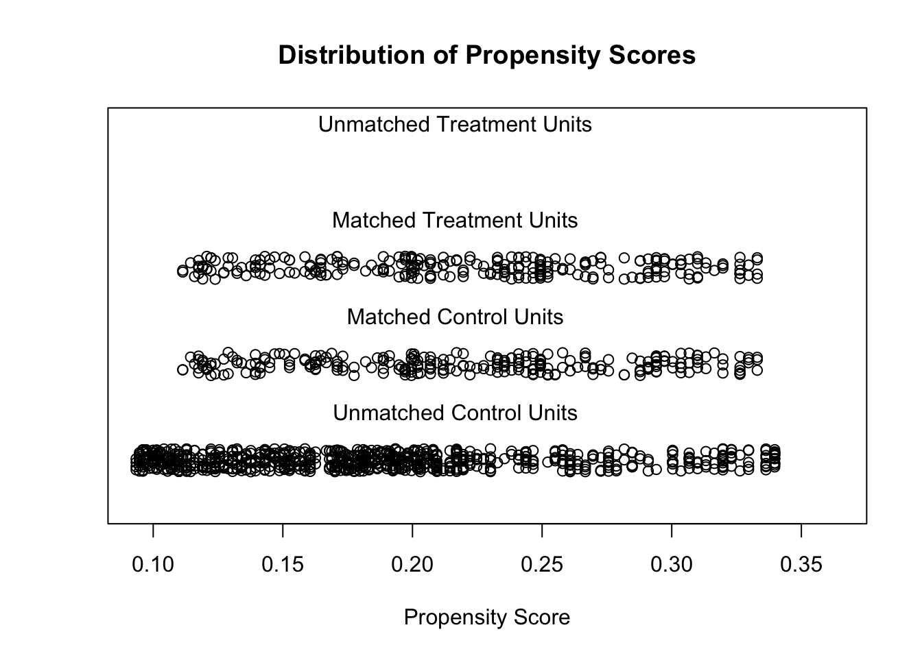

保存匹配样本

df.match <- match.data(match.it)[1:ncol(mydata)]
rm(df.patients, df.population)

Eventually, we can check whether the differences in the level of distress between both samples are still significant.

pacman::p_load(tableone)
table4 <- CreateTableOne(vars = c('Age', 'Sex', 'Distress'), 
                         data = df.match, 
                         factorVars = 'Sex', 
                         strata = 'Sample')
table4 <- print(table4, 
                printToggle = FALSE, 
                noSpaces = TRUE)
knitr::kable(table4[,1:3],  
      align = 'c', 
      caption = 'Table 4: Comparison of matched samples')

Table 4: Table 4: Comparison of matched samples

	Patients	Population	p
n	250	250
Age (mean (SD))	53.51 (13.86)	53.47 (13.85)	0.974
Sex = Female (%)	87 (34.8)	87 (34.8)	1.000
Distress (mean (SD))	23.53 (11.94)	23.68 (11.85)	0.884

With a p-value of 0.222, Student’s t-test does not indicate significant differences anymore. Thus, PSM helped to avoid an alpha mistake.

library(dplyr)
#> 
#> Attaching package: 'dplyr'
#> The following object is masked from 'package:wakefield':
#> 
#>     id
#> The following objects are masked from 'package:stats':
#> 
#>     filter, lag
#> The following objects are masked from 'package:base':
#> 
#>     intersect, setdiff, setequal, union
library(ggplot2)
library(MatchIt)

ecls = read.csv("../../../static/datasets/ecls.csv")

使用非匹配数据进行预分析

ecls %>%
  group_by(catholic) %>%
  summarise(n_students = n(),
            mean_math = mean(c5r2mtsc_std),
            std_error = sd(c5r2mtsc_std) / sqrt(n_students))
#> `summarise()` ungrouping output (override with `.groups` argument)
#> # A tibble: 2 x 4
#>   catholic n_students mean_math std_error
#>      <int>      <int>     <dbl>     <dbl>
#> 1        0       9568   -0.0306    0.0104
#> 2        1       1510    0.194     0.0224

ecls %>%
  mutate(test = (c5r2mtsc - mean(c5r2mtsc)) / sd(c5r2mtsc)) %>% #this is how the math score is standardized
  group_by(catholic) %>%
  summarise(mean_math = mean(test))
#> `summarise()` ungrouping output (override with `.groups` argument)
#> # A tibble: 2 x 2
#>   catholic mean_math
#>      <int>     <dbl>
#> 1        0   -0.0306
#> 2        1    0.194

检验差异：

with(ecls, t.test(c5r2mtsc_std ~ catholic))
#> 
#>  Welch Two Sample t-test
#> 
#> data:  c5r2mtsc_std by catholic
#> t = -9, df = 2215, p-value <2e-16
#> alternative hypothesis: true difference in means is not equal to 0
#> 95 percent confidence interval:
#>  -0.273 -0.176
#> sample estimates:
#> mean in group 0 mean in group 1 
#>         -0.0306          0.1939

协变量探索

We’ll work with the following covariates for now:

• race_white: Is the student white (1) or not (0)?
• p5hmage: Mother’s age
• w3income: Family income
• p5numpla: Number of places the student has lived for at least 4 months
• w3momed_hsb: Is the mother’s education level high-school or below (1) or some college or more (0)?

Let’s calculate the mean for each covariate by the treatment status:

ecls_cov <- c('race_white', 'p5hmage', 'p5numpla', 'w3momed_hsb')
ecls %>%
  group_by(catholic) %>%
  select(one_of(ecls_cov)) %>%
  summarise_all(funs(mean(., na.rm = T)))
#> Adding missing grouping variables: `catholic`
#> Warning: `funs()` is deprecated as of dplyr 0.8.0.
#> Please use a list of either functions or lambdas: 
#> 
#>   # Simple named list: 
#>   list(mean = mean, median = median)
#> 
#>   # Auto named with `tibble::lst()`: 
#>   tibble::lst(mean, median)
#> 
#>   # Using lambdas
#>   list(~ mean(., trim = .2), ~ median(., na.rm = TRUE))
#> This warning is displayed once every 8 hours.
#> Call `lifecycle::last_warnings()` to see where this warning was generated.
#> # A tibble: 2 x 5
#>   catholic race_white p5hmage p5numpla w3momed_hsb
#>      <int>      <dbl>   <dbl>    <dbl>       <dbl>
#> 1        0          0    37.6     1.13           0
#> 2        1          0    39.6     1.09           0

检验：

lapply(ecls_cov, function(v) {
    t.test(ecls[, v] ~ ecls[, 'catholic'])
})
#> [[1]]
#> 
#>  Welch Two Sample t-test
#> 
#> data:  ecls[, v] by ecls[, "catholic"]
#> t = NaN, df = NaN, p-value = NA
#> alternative hypothesis: true difference in means is not equal to 0
#> 95 percent confidence interval:
#>  NaN NaN
#> sample estimates:
#> mean in group 0 mean in group 1 
#>               0               0 
#> 
#> 
#> [[2]]
#> 
#>  Welch Two Sample t-test
#> 
#> data:  ecls[, v] by ecls[, "catholic"]
#> t = -13, df = 2187, p-value <2e-16
#> alternative hypothesis: true difference in means is not equal to 0
#> 95 percent confidence interval:
#>  -2.33 -1.70
#> sample estimates:
#> mean in group 0 mean in group 1 
#>            37.6            39.6 
#> 
#> 
#> [[3]]
#> 
#>  Welch Two Sample t-test
#> 
#> data:  ecls[, v] by ecls[, "catholic"]
#> t = 4, df = 2234, p-value = 2e-05
#> alternative hypothesis: true difference in means is not equal to 0
#> 95 percent confidence interval:
#>  0.0215 0.0584
#> sample estimates:
#> mean in group 0 mean in group 1 
#>            1.13            1.09 
#> 
#> 
#> [[4]]
#> 
#>  Welch Two Sample t-test
#> 
#> data:  ecls[, v] by ecls[, "catholic"]
#> t = NaN, df = NaN, p-value = NA
#> alternative hypothesis: true difference in means is not equal to 0
#> 95 percent confidence interval:
#>  NaN NaN
#> sample estimates:
#> mean in group 0 mean in group 1 
#>               0               0

倾向分估计

m_ps <- glm(catholic ~ race_white + p5hmage + p5numpla + w3momed_hsb,
            family = binomial(), data = ecls)
summary(m_ps)
#> 
#> Call:
#> glm(formula = catholic ~ race_white + p5hmage + p5numpla + w3momed_hsb, 
#>     family = binomial(), data = ecls)
#> 
#> Deviance Residuals: 
#>    Min      1Q  Median      3Q     Max  
#> -1.166  -0.587  -0.528  -0.463   2.305  
#> 
#> Coefficients: (2 not defined because of singularities)
#>             Estimate Std. Error z value Pr(>|z|)    
#> (Intercept) -3.28365    0.20921  -15.70   <2e-16 ***
#> race_white        NA         NA      NA       NA    
#> p5hmage      0.04582    0.00444   10.33   <2e-16 ***
#> p5numpla    -0.22521    0.09059   -2.49    0.013 *  
#> w3momed_hsb       NA         NA      NA       NA    
#> ---
#> Signif. codes:  0 '***' 0.001 '**' 0.01 '*' 0.05 '.' 0.1 ' ' 1
#> 
#> (Dispersion parameter for binomial family taken to be 1)
#> 
#>     Null deviance: 7701.3  on 9266  degrees of freedom
#> Residual deviance: 7583.5  on 9264  degrees of freedom
#>   (1811 observations deleted due to missingness)
#> AIC: 7589
#> 
#> Number of Fisher Scoring iterations: 4

prs_df <- data.frame(pr_score = predict(m_ps, type = "response"),
                     catholic = m_ps$model$catholic)
head(prs_df)
#>   pr_score catholic
#> 1    0.205        0
#> 2    0.164        0
#> 4    0.177        0
#> 5    0.146        1
#> 6    0.205        0
#> 7    0.106        0
labs <- paste("Actual school type attended:", c("Catholic", "Public"))
prs_df %>%
  mutate(catholic = ifelse(catholic == 1, labs[1], labs[2])) %>%
  ggplot(aes(x = pr_score)) +
  geom_histogram(color = "white") +
  facet_wrap(~catholic) +
  xlab("Probability of going to Catholic school") +
  theme_bw()
#> `stat_bin()` using `bins = 30`. Pick better value with `binwidth`.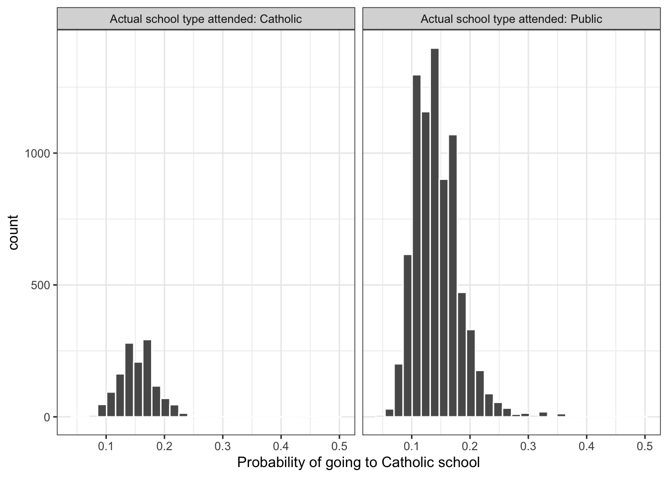

执行匹配算法

ecls_nomiss <- ecls %>%  # MatchIt does not allow missing values
  select(c5r2mtsc_std, catholic, one_of(ecls_cov)) %>%
  na.omit()
mod_match <- matchit(catholic ~ race_white + p5hmage + p5numpla + w3momed_hsb,
                     method = "nearest", data = ecls_nomiss)

dta_m <- match.data(mod_match)
dim(dta_m)
#> [1] 2704    8

检查匹配样本中协变量的平衡

fn_bal <- function(dta, variable) {
  dta$variable <- dta[, variable]
  if (variable == 'w3income') dta$variable <- dta$variable / 10^3
  dta$catholic <- as.factor(dta$catholic)
  support <- c(min(dta$variable), max(dta$variable))
  ggplot(dta, aes(x = distance, y = variable, color = catholic)) +
    geom_point(alpha = 0.2, size = 1.3) +
    geom_smooth(method = "loess", se = F) +
    xlab("Propensity score") +
    ylab(variable) +
    theme_bw() +
    ylim(support)
}
library(gridExtra)
#> 
#> Attaching package: 'gridExtra'
#> The following object is masked from 'package:dplyr':
#> 
#>     combine
grid.arrange(
   fn_bal(dta_m, "p5numpla") + theme(legend.position = "none"),
   fn_bal(dta_m, "p5hmage"),
   fn_bal(dta_m, "w3momed_hsb") + theme(legend.position = "none"),
   fn_bal(dta_m, "race_white"),
   nrow = 2, widths = c(1, 0.8)
)
#> `geom_smooth()` using formula 'y ~ x'
#> Warning: Removed 41 rows containing missing values (geom_smooth).
#> `geom_smooth()` using formula 'y ~ x'
#> Warning: Removed 1 rows containing missing values (geom_smooth).
#> `geom_smooth()` using formula 'y ~ x'
#> `geom_smooth()` using formula 'y ~ x'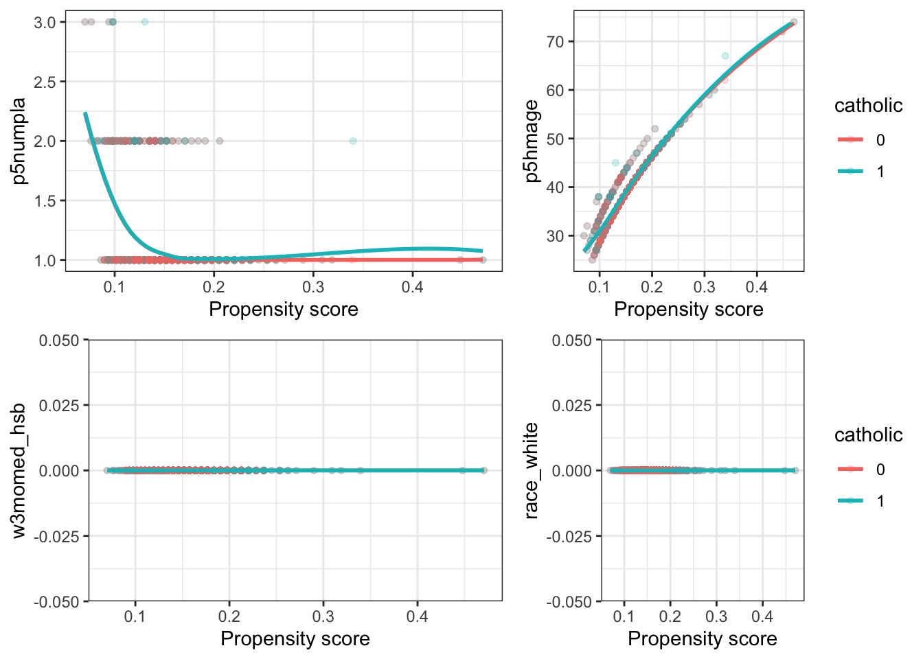

均值差异

dta_m %>%
  group_by(catholic) %>%
  select(one_of(ecls_cov)) %>%
  summarise_all(funs(mean))
#> Adding missing grouping variables: `catholic`
#> # A tibble: 2 x 5
#>   catholic race_white p5hmage p5numpla w3momed_hsb
#>      <int>      <dbl>   <dbl>    <dbl>       <dbl>
#> 1        0          0    39.6     1.09           0
#> 2        1          0    39.6     1.09           0

检验：

lapply(ecls_cov, function(v) {
    t.test(dta_m[, v] ~ dta_m$catholic)
})
#> [[1]]
#> 
#>  Welch Two Sample t-test
#> 
#> data:  dta_m[, v] by dta_m$catholic
#> t = NaN, df = NaN, p-value = NA
#> alternative hypothesis: true difference in means is not equal to 0
#> 95 percent confidence interval:
#>  NaN NaN
#> sample estimates:
#> mean in group 0 mean in group 1 
#>               0               0 
#> 
#> 
#> [[2]]
#> 
#>  Welch Two Sample t-test
#> 
#> data:  dta_m[, v] by dta_m$catholic
#> t = -0.06, df = 2702, p-value = 1
#> alternative hypothesis: true difference in means is not equal to 0
#> 95 percent confidence interval:
#>  -0.405  0.383
#> sample estimates:
#> mean in group 0 mean in group 1 
#>            39.6            39.6 
#> 
#> 
#> [[3]]
#> 
#>  Welch Two Sample t-test
#> 
#> data:  dta_m[, v] by dta_m$catholic
#> t = -0.2, df = 2700, p-value = 0.8
#> alternative hypothesis: true difference in means is not equal to 0
#> 95 percent confidence interval:
#>  -0.0250  0.0206
#> sample estimates:
#> mean in group 0 mean in group 1 
#>            1.09            1.09 
#> 
#> 
#> [[4]]
#> 
#>  Welch Two Sample t-test
#> 
#> data:  dta_m[, v] by dta_m$catholic
#> t = NaN, df = NaN, p-value = NA
#> alternative hypothesis: true difference in means is not equal to 0
#> 95 percent confidence interval:
#>  NaN NaN
#> sample estimates:
#> mean in group 0 mean in group 1 
#>               0               0

Average absolute standardized difference

As a measure of the average imbalance, we can calculate the following:

\[\bar{\left|\frac{\beta}{\sigma}\right|} = \frac{1}{k}\sum_x \frac{|\beta_x|}{\sigma_x}\]

where βx is the difference between the covariate means in the treated and control groups in the matched sample. An average absolute standardized difference that is close to 0 is preferable, since that indicates small differences between the control and treatment groups in the matched sample.

Try to implement a function that calculates the absolute standardized difference for any covariate in the matched sample. Then take the average for all the covariates.

评估治疗效应

Estimating the treatment effect is simple once we have a matched sample that we are happy with. We can use a t-test，Or we can use OLS with or without covariates。

---

资料来源：

• https://www.r-bloggers.com/how-to-use-r-for-matching-samples-propensity-score/
• https://sejdemyr.github.io/r-tutorials/statistics/tutorial8.html