R 语言统计检验函数汇总
王诗翔 · 2019-12-25
资料来源:《R 语言核心技术手册》和 R 文档
数据基本来自胡编乱造 和 R 文档
本文基本囊括了常用的统计检验在 R 中的实现函数和使用方法。
连续型数据
基于正态分布的检验
均值检验
t.test(1:10, 10:20)
#>
#>  Welch Two Sample t-test
#>
#> data:  1:10 and 10:20
#> t = -7, df = 19, p-value = 2e-06
#> alternative hypothesis: true difference in means is not equal to 0
#> 95 percent confidence interval:
#>  -12.4  -6.6
#> sample estimates:
#> mean of x mean of y
#>       5.5      15.0
配对 t 检验:
t.test(rnorm(10), rnorm(10, mean = 1), paired = TRUE)
#>
#>  Paired t-test
#>
#> data:  rnorm(10) and rnorm(10, mean = 1)
#> t = -2, df = 9, p-value = 0.09
#> alternative hypothesis: true difference in means is not equal to 0
#> 95 percent confidence interval:
#>  -1.419  0.134
#> sample estimates:
#> mean of the differences
#>                  -0.643
使用公式:
df <- data.frame(
  value = c(rnorm(10), rnorm(10, mean = 1)),
  group = c(rep("control", 10), rep("test", 10))
)

t.test(value ~ group, data = df)
#>
#>  Welch Two Sample t-test
#>
#> data:  value by group
#> t = -2, df = 16, p-value = 0.03
#> alternative hypothesis: true difference in means is not equal to 0
#> 95 percent confidence interval:
#>  -1.7767 -0.0945
#> sample estimates:
#> mean in group control    mean in group test
#>                 0.314                 1.250
假设方差同质:
t.test(value ~ group, data = df, var.equal = TRUE)
#>
#>  Two Sample t-test
#>
#> data:  value by group
#> t = -2, df = 18, p-value = 0.03
#> alternative hypothesis: true difference in means is not equal to 0
#> 95 percent confidence interval:
#>  -1.768 -0.103
#> sample estimates:
#> mean in group control    mean in group test
#>                 0.314                 1.250
更多查看 ?t.test。
两总体方差检验
上面的例子假设方差同质,我们通过检验查看。
服从正态分布的两总体方差比较。
# 进行的是 F 检验
var.test(value ~ group, data = df)
#>
#>  F test to compare two variances
#>
#> data:  value by group
#> F = 2, num df = 9, denom df = 9, p-value = 0.3
#> alternative hypothesis: true ratio of variances is not equal to 1
#> 95 percent confidence interval:
#>  0.546 8.846
#> sample estimates:
#> ratio of variances
#>                2.2
使用 Bartlett 检验比较每个组(样本)数据的方差是否一致。
bartlett.test(value ~ group, data = df)
#>
#>  Bartlett test of homogeneity of variances
#>
#> data:  value by group
#> Bartlett's K-squared = 1, df = 1, p-value = 0.3
多个组间均值的比较
对于两组以上数据间均值的比较,使用方差分析 ANOVA。
aov(wt ~ factor(cyl), data = mtcars)
#> Call:
#>    aov(formula = wt ~ factor(cyl), data = mtcars)
#>
#> Terms:
#>                 factor(cyl) Residuals
#> Sum of Squares         18.2      11.5
#> Deg. of Freedom           2        29
#>
#> Residual standard error: 0.63
#> Estimated effects may be unbalanced
查看详细信息:
model.tables(aov(wt ~ factor(cyl), data = mtcars))
#> Tables of effects
#>
#>  factor(cyl)
#>           4       6      8
#>     -0.9315 -0.1001  0.782
#> rep 11.0000  7.0000 14.000
通常先用 lm() 函数对数据建立线性模型,再用 anova() 函数提取方差分析的信息更方便。
md <- lm(wt ~ factor(cyl), data = mtcars)
anova(md)
#> Analysis of Variance Table
#>
#> Response: wt
#>             Df Sum Sq Mean Sq F value  Pr(>F)
#> factor(cyl)  2   18.2    9.09    22.9 1.1e-06 ***
#> Residuals   29   11.5    0.40
#> ---
#> Signif. codes:  0 '***' 0.001 '**' 0.01 '*' 0.05 '.' 0.1 ' ' 1
ANOVA 分析假设各组样本数据的方差是相等的,如果知道(或怀疑)不相等,可以使用 oneway.test() 函数。
oneway.test(wt ~ cyl, data = mtcars)
#>
#>  One-way analysis of means (not assuming equal variances)
#>
#> data:  wt and cyl
#> F = 20, num df = 2, denom df = 19, p-value = 2e-05
这与设定了 var.equal=FALSE 的 t.test 类似(两种方法都是 Welch 提出)。
多组样本的配对 t 检验
pairwise.t.test(mtcars$wt, mtcars$cyl)
#>
#>  Pairwise comparisons using t tests with pooled SD
#>
#> data:  mtcars$wt and mtcars$cyl
#>
#>   4     6
#> 6 0.01  -
#> 8 6e-07 0.01
#>
#> P value adjustment method: holm
可以自定义 p 值校正方法。
正态性检验
使用 Shapiro-Wilk 检验:
shapiro.test(rnorm(30))
#>
#>  Shapiro-Wilk normality test
#>
#> data:  rnorm(30)
#> W = 1, p-value = 0.7
可以通过 QQ 图辅助查看。
qqnorm(rnorm(30))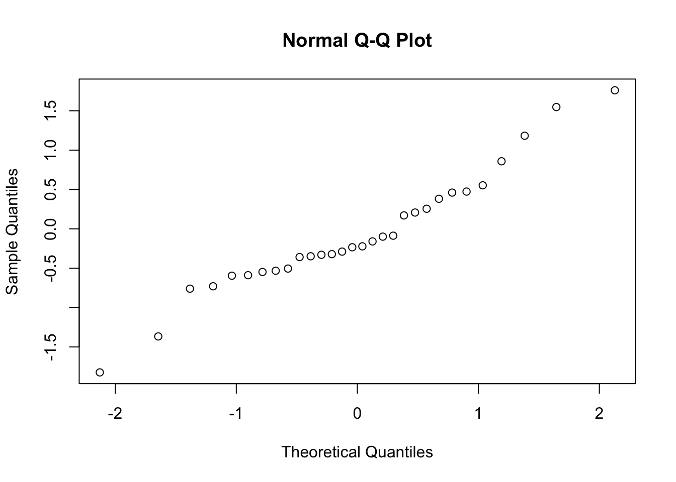
分布的对称性检验
用 Kolmogorov-Smirnov 检验查看一个向量是否来自对称的概率分布(不限于正态分布)。
ks.test(rnorm(10), pnorm)
#>
#>  One-sample Kolmogorov-Smirnov test
#>
#> data:  rnorm(10)
#> D = 0.2, p-value = 0.8
#> alternative hypothesis: two-sided
函数第 1 个参数指定待检验的数据,第 2 个参数指定对称分布的类型,可以是数值型向量、指定概率分布函数的字符串或一个分布函数。
ks.test(rnorm(10), "pnorm")
#>
#>  One-sample Kolmogorov-Smirnov test
#>
#> data:  rnorm(10)
#> D = 0.4, p-value = 0.1
#> alternative hypothesis: two-sided

ks.test(rpois(10, lambda = 1), "pnorm")
#> Warning in ks.test(rpois(10, lambda = 1), "pnorm"): ties should not be present
#> for the Kolmogorov-Smirnov test
#>
#>  One-sample Kolmogorov-Smirnov test
#>
#> data:  rpois(10, lambda = 1)
#> D = 0.6, p-value = 5e-04
#> alternative hypothesis: two-sided
检验两个向量是否服从同一分布
还是用上面的函数。
ks.test(rnorm(20), rnorm(30))
#>
#>  Two-sample Kolmogorov-Smirnov test
#>
#> data:  rnorm(20) and rnorm(30)
#> D = 0.2, p-value = 0.8
#> alternative hypothesis: two-sided
相关性检验
使用 cor.test() 函数。
cor.test(mtcars$mpg, mtcars$wt)
#>
#>  Pearson's product-moment correlation
#>
#> data:  mtcars$mpg and mtcars$wt
#> t = -10, df = 30, p-value = 1e-10
#> alternative hypothesis: true correlation is not equal to 0
#> 95 percent confidence interval:
#>  -0.934 -0.744
#> sample estimates:
#>    cor
#> -0.868
一共有 3 种方法,具体看选项 method 的说明。
cor.test(mtcars$mpg, mtcars$wt, method = "spearman", exact = F)
#>
#>  Spearman's rank correlation rho
#>
#> data:  mtcars$mpg and mtcars$wt
#> S = 10292, p-value = 1e-11
#> alternative hypothesis: true rho is not equal to 0
#> sample estimates:
#>    rho
#> -0.886
不依赖分布的检验
均值检验
Wilcoxon 检验是 t 检验的非参数版本。
默认是秩和检验。
wilcox.test(1:10, 10:20)
#> Warning in wilcox.test.default(1:10, 10:20): cannot compute exact p-value with
#> ties
#>
#>  Wilcoxon rank sum test with continuity correction
#>
#> data:  1:10 and 10:20
#> W = 0.5, p-value = 1e-04
#> alternative hypothesis: true location shift is not equal to 0
可以设定为符号检验。
wilcox.test(1:10, 10:19, paired = TRUE)
#> Warning in wilcox.test.default(1:10, 10:19, paired = TRUE): cannot compute exact
#> p-value with ties
#>
#>  Wilcoxon signed rank test with continuity correction
#>
#> data:  1:10 and 10:19
#> V = 0, p-value = 0.002
#> alternative hypothesis: true location shift is not equal to 0
多均值比较
多均值比较使 Kruskal-Wallis 秩和检验。
kruskal.test(wt ~ factor(cyl), data = mtcars)
#>
#>  Kruskal-Wallis rank sum test
#>
#> data:  wt by factor(cyl)
#> Kruskal-Wallis chi-squared = 23, df = 2, p-value = 1e-05
方差检验
使用Fligner-Killeen(中位数)检验完成不同组别的方差比较
fligner.test(wt ~ cyl, data = mtcars)
#>
#>  Fligner-Killeen test of homogeneity of variances
#>
#> data:  wt by cyl
#> Fligner-Killeen:med chi-squared = 0.5, df = 2, p-value = 0.8
尺度参数差异
R 有一些检验可以用来确定尺度参数的差异。分布的尺度参数确定分布函数的尺度,如 t 分布的自由度。
下面是针对两样本尺度参数差异的 Ansari-Bradley 检验。
## Hollander & Wolfe (1973, p. 86f):
## Serum iron determination using Hyland control sera
ramsay <- c(111, 107, 100, 99, 102, 106, 109, 108, 104, 99,
            101, 96, 97, 102, 107, 113, 116, 113, 110, 98)
jung.parekh <- c(107, 108, 106, 98, 105, 103, 110, 105, 104,
            100, 96, 108, 103, 104, 114, 114, 113, 108, 106, 99)
ansari.test(ramsay, jung.parekh)
#> Warning in ansari.test.default(ramsay, jung.parekh): cannot compute exact p-
#> value with ties
#>
#>  Ansari-Bradley test
#>
#> data:  ramsay and jung.parekh
#> AB = 186, p-value = 0.2
#> alternative hypothesis: true ratio of scales is not equal to 1
还可以使用 Mood 两样本检验做。
mood.test(ramsay, jung.parekh)
#>
#>  Mood two-sample test of scale
#>
#> data:  ramsay and jung.parekh
#> Z = 1, p-value = 0.3
#> alternative hypothesis: two.sided
离散数据
比例检验
使用 prop.test() 比较两组观测值发生的概率是否有差异。
heads <- rbinom(1, size = 100, prob = .5)
prop.test(heads, 100)          # continuity correction TRUE by default
#>
#>  1-sample proportions test with continuity correction
#>
#> data:  heads out of 100, null probability 0.5
#> X-squared = 0.01, df = 1, p-value = 0.9
#> alternative hypothesis: true p is not equal to 0.5
#> 95 percent confidence interval:
#>  0.409 0.611
#> sample estimates:
#>    p
#> 0.51
prop.test(heads, 100, correct = FALSE)
#>
#>  1-sample proportions test without continuity correction
#>
#> data:  heads out of 100, null probability 0.5
#> X-squared = 0.04, df = 1, p-value = 0.8
#> alternative hypothesis: true p is not equal to 0.5
#> 95 percent confidence interval:
#>  0.413 0.606
#> sample estimates:
#>    p
#> 0.51
可以给定概率值。
prop.test(heads, 100, p = 0.3, correct = FALSE)
#>
#>  1-sample proportions test without continuity correction
#>
#> data:  heads out of 100, null probability 0.3
#> X-squared = 21, df = 1, p-value = 5e-06
#> alternative hypothesis: true p is not equal to 0.3
#> 95 percent confidence interval:
#>  0.413 0.606
#> sample estimates:
#>    p
#> 0.51
二项式检验
binom.test(c(682, 243), p = 3/4)
#>
#>  Exact binomial test
#>
#> data:  c(682, 243)
#> number of successes = 682, number of trials = 925, p-value = 0.4
#> alternative hypothesis: true probability of success is not equal to 0.75
#> 95 percent confidence interval:
#>  0.708 0.765
#> sample estimates:
#> probability of success
#>                  0.737
binom.test(682, 682 + 243, p = 3/4)  # The same
#>
#>  Exact binomial test
#>
#> data:  682 and 682 + 243
#> number of successes = 682, number of trials = 925, p-value = 0.4
#> alternative hypothesis: true probability of success is not equal to 0.75
#> 95 percent confidence interval:
#>  0.708 0.765
#> sample estimates:
#> probability of success
#>                  0.737
与其他的检验函数不同,这里的 p 值表示试验成功率与假设值的最小差值。
列联表检验
用来确定两个分类变量是否相关。
对于小的列联表,试验 Fisher 精确检验获得较好的检验结果。
Fisher 检验有一个关于喝茶的故事。
## Agresti (1990, p. 61f; 2002, p. 91) Fisher's Tea Drinker
## A British woman claimed to be able to distinguish whether milk or
##  tea was added to the cup first.  To test, she was given 8 cups of
##  tea, in four of which milk was added first.  The null hypothesis
##  is that there is no association between the true order of pouring
##  and the woman's guess, the alternative that there is a positive
##  association (that the odds ratio is greater than 1).
TeaTasting <-
matrix(c(3, 1, 1, 3),
       nrow = 2,
       dimnames = list(Guess = c("Milk", "Tea"),
                       Truth = c("Milk", "Tea")))
fisher.test(TeaTasting, alternative = "greater")
#>
#>  Fisher's Exact Test for Count Data
#>
#> data:  TeaTasting
#> p-value = 0.2
#> alternative hypothesis: true odds ratio is greater than 1
#> 95 percent confidence interval:
#>  0.314   Inf
#> sample estimates:
#> odds ratio
#>       6.41
## => p = 0.2429, association could not be established
当列联表较大时,Fisher 计算量很大,可以使用卡方检验替代。
chisq.test(TeaTasting)
#> Warning in chisq.test(TeaTasting): Chi-squared approximation may be incorrect
#>
#>  Pearson's Chi-squared test with Yates' continuity correction
#>
#> data:  TeaTasting
#> X-squared = 0.5, df = 1, p-value = 0.5
对于三变量的混合影响,使用 Cochran-Mantel-Haenszel 检验。
## Agresti (1990), pages 231--237, Penicillin and Rabbits
## Investigation of the effectiveness of immediately injected or 1.5
##  hours delayed penicillin in protecting rabbits against a lethal
##  injection with beta-hemolytic streptococci.
Rabbits <-
array(c(0, 0, 6, 5,
        3, 0, 3, 6,
        6, 2, 0, 4,
        5, 6, 1, 0,
        2, 5, 0, 0),
      dim = c(2, 2, 5),
      dimnames = list(
          Delay = c("None", "1.5h"),
          Response = c("Cured", "Died"),
          Penicillin.Level = c("1/8", "1/4", "1/2", "1", "4")))
Rabbits
#> , , Penicillin.Level = 1/8
#>
#>       Response
#> Delay  Cured Died
#>   None     0    6
#>   1.5h     0    5
#>
#> , , Penicillin.Level = 1/4
#>
#>       Response
#> Delay  Cured Died
#>   None     3    3
#>   1.5h     0    6
#>
#> , , Penicillin.Level = 1/2
#>
#>       Response
#> Delay  Cured Died
#>   None     6    0
#>   1.5h     2    4
#>
#> , , Penicillin.Level = 1
#>
#>       Response
#> Delay  Cured Died
#>   None     5    1
#>   1.5h     6    0
#>
#> , , Penicillin.Level = 4
#>
#>       Response
#> Delay  Cured Died
#>   None     2    0
#>   1.5h     5    0
## Classical Mantel-Haenszel test
mantelhaen.test(Rabbits)
#>
#>  Mantel-Haenszel chi-squared test with continuity correction
#>
#> data:  Rabbits
#> Mantel-Haenszel X-squared = 4, df = 1, p-value = 0.05
#> alternative hypothesis: true common odds ratio is not equal to 1
#> 95 percent confidence interval:
#>   1.03 47.73
#> sample estimates:
#> common odds ratio
#>                 7
用 McNemar 卡方检验检验二维列联表的对称性。
## Agresti (1990), p. 350.
## Presidential Approval Ratings.
##  Approval of the President's performance in office in two surveys,
##  one month apart, for a random sample of 1600 voting-age Americans.
Performance <-
matrix(c(794, 86, 150, 570),
       nrow = 2,
       dimnames = list("1st Survey" = c("Approve", "Disapprove"),
                       "2nd Survey" = c("Approve", "Disapprove")))
Performance
#>             2nd Survey
#> 1st Survey   Approve Disapprove
#>   Approve        794        150
#>   Disapprove      86        570
mcnemar.test(Performance)
#>
#>  McNemar's Chi-squared test with continuity correction
#>
#> data:  Performance
#> McNemar's chi-squared = 17, df = 1, p-value = 4e-05
列联表非参数检验
Friedman 秩和检验是一个非参数版本的双边 ANOVA 检验。
## Hollander & Wolfe (1973), p. 140ff.
## Comparison of three methods ("round out", "narrow angle", and
##  "wide angle") for rounding first base.  For each of 18 players
##  and the three method, the average time of two runs from a point on
##  the first base line 35ft from home plate to a point 15ft short of
##  second base is recorded.
RoundingTimes <-
matrix(c(5.40, 5.50, 5.55,
         5.85, 5.70, 5.75,
         5.20, 5.60, 5.50,
         5.55, 5.50, 5.40,
         5.90, 5.85, 5.70,
         5.45, 5.55, 5.60,
         5.40, 5.40, 5.35,
         5.45, 5.50, 5.35,
         5.25, 5.15, 5.00,
         5.85, 5.80, 5.70,
         5.25, 5.20, 5.10,
         5.65, 5.55, 5.45,
         5.60, 5.35, 5.45,
         5.05, 5.00, 4.95,
         5.50, 5.50, 5.40,
         5.45, 5.55, 5.50,
         5.55, 5.55, 5.35,
         5.45, 5.50, 5.55,
         5.50, 5.45, 5.25,
         5.65, 5.60, 5.40,
         5.70, 5.65, 5.55,
         6.30, 6.30, 6.25),
       nrow = 22,
       byrow = TRUE,
       dimnames = list(1 : 22,
                       c("Round Out", "Narrow Angle", "Wide Angle")))
friedman.test(RoundingTimes)
#>
#>  Friedman rank sum test
#>
#> data:  RoundingTimes
#> Friedman chi-squared = 11, df = 2, p-value = 0.004