Forest Plot(森林图)绘制
王诗翔 · 2018-09-10
分类:
r
标签:
r
forestplot
森林图常见于元分析,但其使用绝不仅如此,比如我现在想要研究的对象有诸多HR结果,我想要汇总为一张图,森林图就是个非常好的选择。ggpubr包提供的森林图是针对变量分析绘图,我也尝试使用了metafor包的forest画图函数,但太灵活了,我除了感觉文档画的不错,但实际使用却很难得到想要的结果。
谷歌了一下,找到了forestplot这个包,下面根据文档学习一波。
安装:
install.packages("forestplot")文本
森林图可以与文本连接起来并自定义。
文本表
下面是一个使用文本表的例子:
library(forestplot)
#> Loading required package: grid
#> Loading required package: magrittr
#> Loading required package: checkmate
# Cochrane data from the 'rmeta'-package
cochrane_from_rmeta <-
  structure(list(
    mean  = c(NA, NA, 0.578, 0.165, 0.246, 0.700, 0.348, 0.139, 1.017, NA, 0.531),
    lower = c(NA, NA, 0.372, 0.018, 0.072, 0.333, 0.083, 0.016, 0.365, NA, 0.386),
    upper = c(NA, NA, 0.898, 1.517, 0.833, 1.474, 1.455, 1.209, 2.831, NA, 0.731)),
    .Names = c("mean", "lower", "upper"),
    row.names = c(NA, -11L),
    class = "data.frame")
tabletext<-cbind(
  c("", "Study", "Auckland", "Block",
    "Doran", "Gamsu", "Morrison", "Papageorgiou",
    "Tauesch", NA, "Summary"),
  c("Deaths", "(steroid)", "36", "1",
    "4", "14", "3", "1",
    "8", NA, NA),
  c("Deaths", "(placebo)", "60", "5",
    "11", "20", "7", "7",
    "10", NA, NA),
  c("", "OR", "0.58", "0.16",
    "0.25", "0.70", "0.35", "0.14",
    "1.02", NA, "0.53"))
forestplot(tabletext,
           cochrane_from_rmeta,new_page = TRUE,
           is.summary=c(TRUE,TRUE,rep(FALSE,8),TRUE),
           clip=c(0.1,2.5),
           xlog=TRUE,
           col=fpColors(box="royalblue",line="darkblue", summary="royalblue"))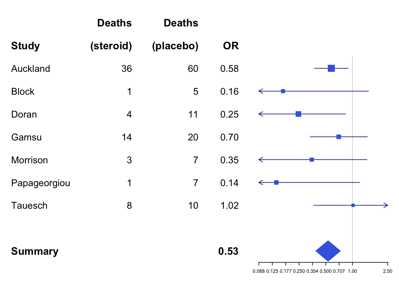
汇总线
在上面基础进行增改:
forestplot(tabletext,
           hrzl_lines = gpar(col="#444444"),
           cochrane_from_rmeta,new_page = TRUE,
           is.summary=c(TRUE,TRUE,rep(FALSE,8),TRUE),
           clip=c(0.1,2.5),
           xlog=TRUE,
           col=fpColors(box="royalblue",line="darkblue", summary="royalblue"))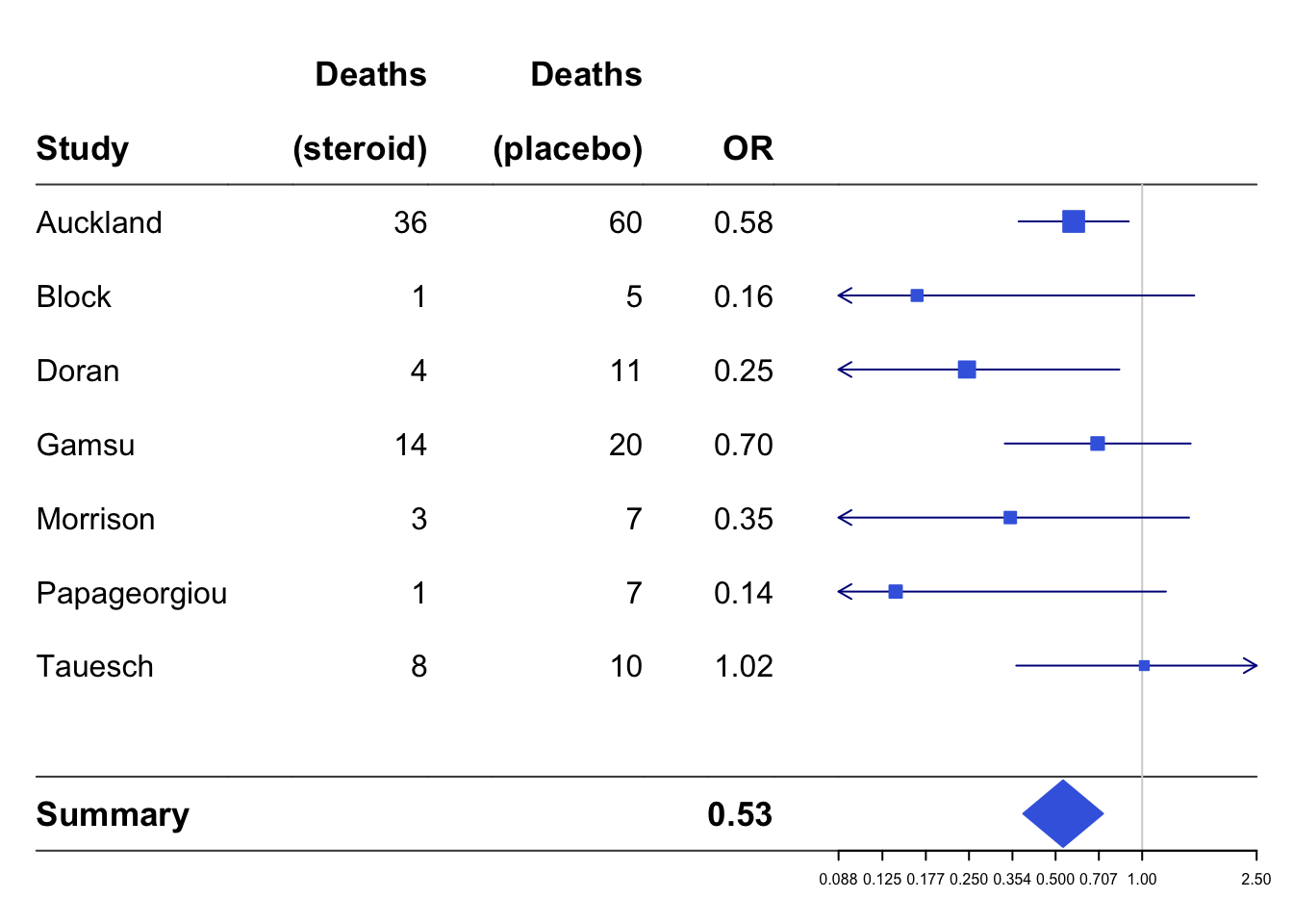
我们可以修改线条类型和它所影响的范围:
forestplot(tabletext,
           hrzl_lines = list("3" = gpar(lty=2),
                             "11" = gpar(lwd=1, columns=1:4, col = "#000044")),
           cochrane_from_rmeta,new_page = TRUE,
           is.summary=c(TRUE,TRUE,rep(FALSE,8),TRUE),
           clip=c(0.1,2.5),
           xlog=TRUE,
           col=fpColors(box="royalblue",line="darkblue", summary="royalblue", hrz_lines = "#444444"))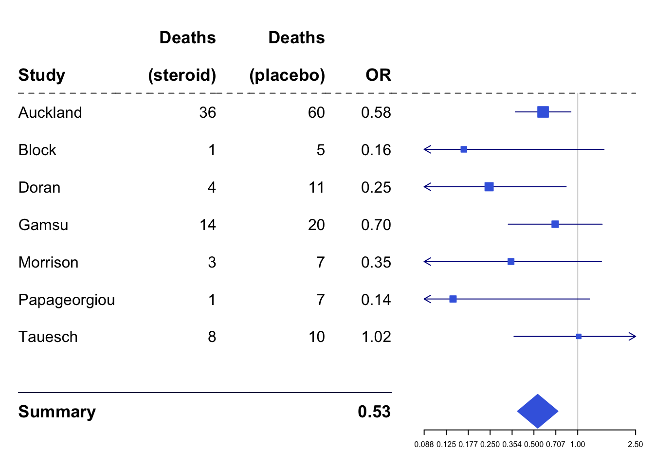
为端点增加垂线:
forestplot(tabletext,
           hrzl_lines = list("3" = gpar(lty=2),
                             "11" = gpar(lwd=1, columns=1:4, col = "#000044")),
           cochrane_from_rmeta,new_page = TRUE,
           is.summary=c(TRUE,TRUE,rep(FALSE,8),TRUE),
           clip=c(0.1,2.5),
           xlog=TRUE,
           col=fpColors(box="royalblue",line="darkblue", summary="royalblue", hrz_lines = "#444444"),
           vertices = TRUE)
调整图元素的位置
forestplot(tabletext,
           graph.pos = 4,
           hrzl_lines = list("3" = gpar(lty=2),
                             "11" = gpar(lwd=1, columns=c(1:3,5), col = "#000044"),
                             "12" = gpar(lwd=1, lty=2, columns=c(1:3,5), col = "#000044")),
           cochrane_from_rmeta,new_page = TRUE,
           is.summary=c(TRUE,TRUE,rep(FALSE,8),TRUE),
           clip=c(0.1,2.5),
           xlog=TRUE,
           col=fpColors(box="royalblue",line="darkblue", summary="royalblue", hrz_lines = "#444444"))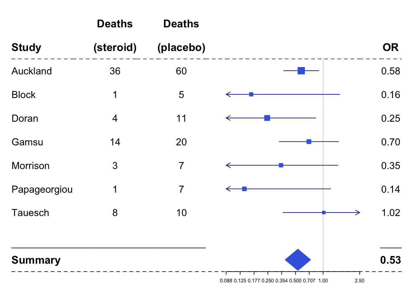
使用表达式
data(HRQoL)
clrs <- fpColors(box="royalblue",line="darkblue", summary="royalblue")
tabletext <-
  list(c(NA, rownames(HRQoL$Sweden)),
       append(list(expression(beta)), sprintf("%.2f", HRQoL$Sweden[,"coef"])))
forestplot(tabletext,
           rbind(rep(NA, 3),
                 HRQoL$Sweden),
           col=clrs,
           xlab="EQ-5D index")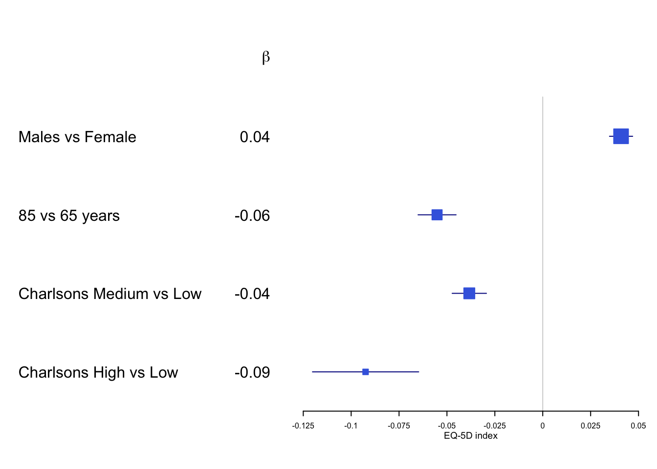
更改字体
tabletext <- cbind(rownames(HRQoL$Sweden),
                   sprintf("%.2f", HRQoL$Sweden[,"coef"]))
forestplot(tabletext,
           txt_gp = fpTxtGp(label = gpar(fontfamily = "HersheyScript")),
           rbind(HRQoL$Sweden),
           col=clrs,
           xlab="EQ-5D index")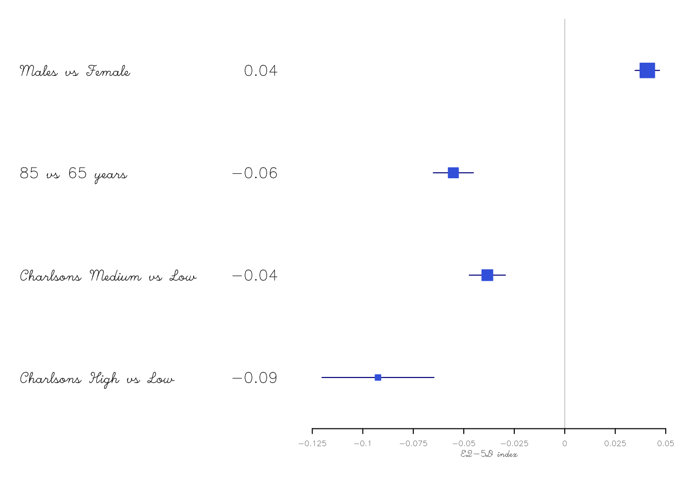
还可以更改风格:
forestplot(tabletext,
           txt_gp = fpTxtGp(label = list(gpar(fontfamily = "HersheyScript"),
                                         gpar(fontfamily = "",
                                              col = "#660000")),
                            ticks = gpar(fontfamily = "", cex=1),
                            xlab  = gpar(fontfamily = "HersheySerif", cex = 1.5)),
           rbind(HRQoL$Sweden),
           col=clrs,
           xlab="EQ-5D index")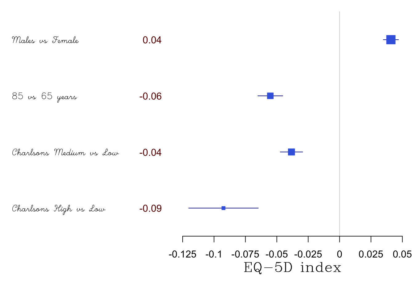
置信区间
简单的,给超出范围的区间加箭头(clip):
forestplot(tabletext,
           rbind(HRQoL$Sweden),
           clip =c(-.1, Inf),
           col=clrs,
           xlab="EQ-5D index")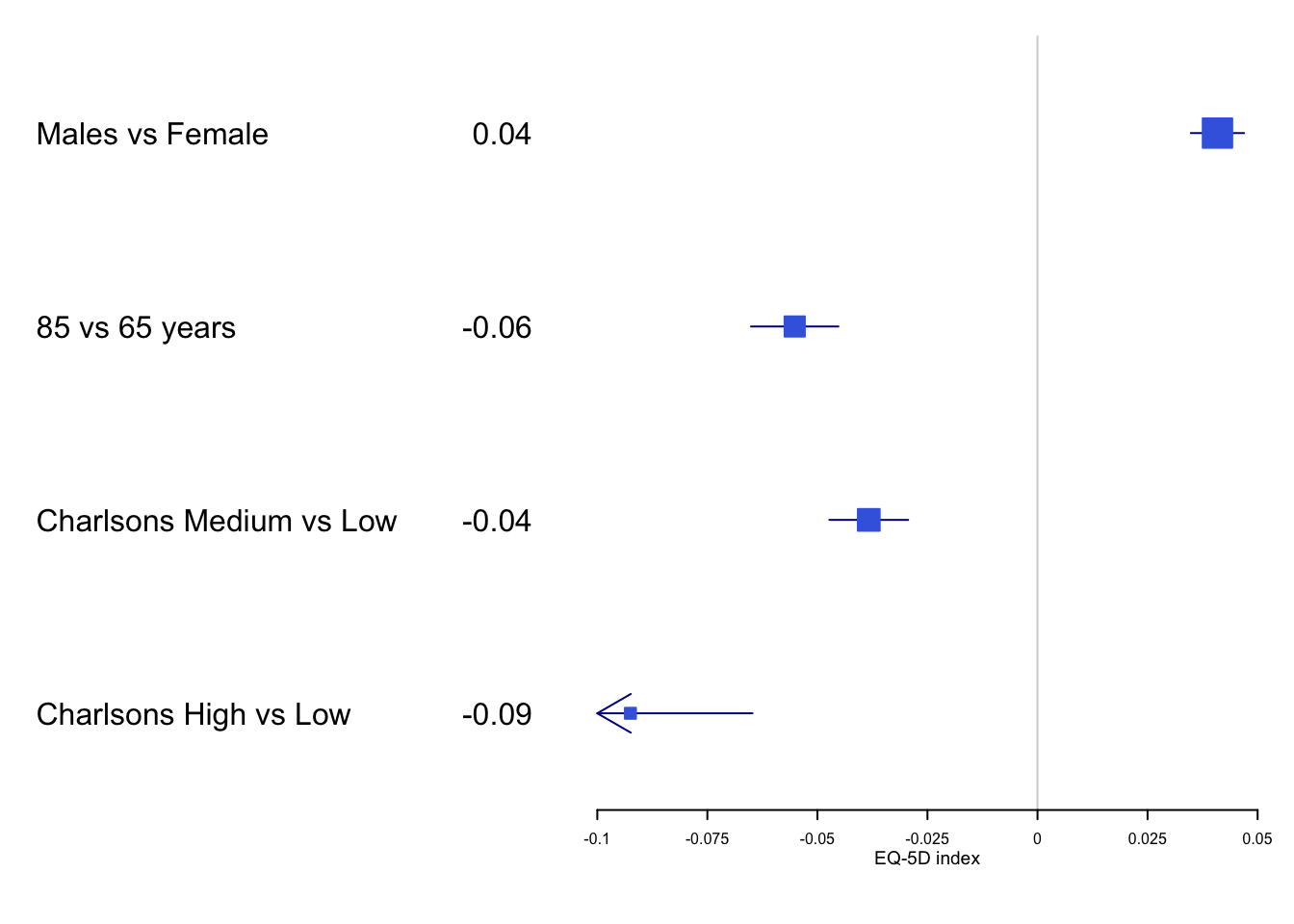
多个置信区间范围
这在对比时非常有用:
tabletext <- tabletext[,1]
forestplot(tabletext,
           mean = cbind(HRQoL$Sweden[, "coef"], HRQoL$Denmark[, "coef"]),
           lower = cbind(HRQoL$Sweden[, "lower"], HRQoL$Denmark[, "lower"]),
           upper = cbind(HRQoL$Sweden[, "upper"], HRQoL$Denmark[, "upper"]),
           clip =c(-.1, 0.075),
           col=fpColors(box=c("blue", "darkred")),
           xlab="EQ-5D index")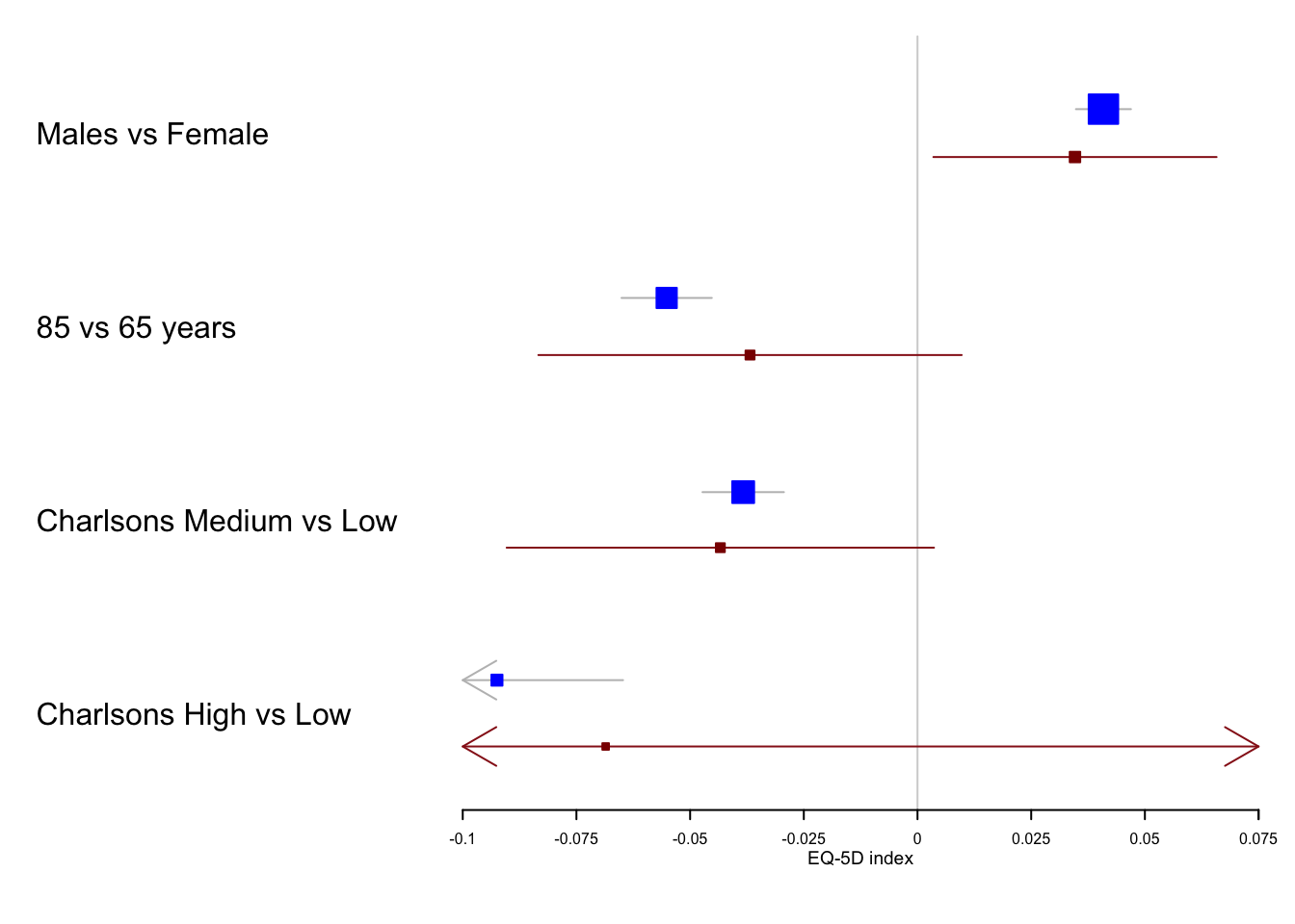
评估显示器
可以用方块、圆圈等:
forestplot(tabletext,
            fn.ci_norm = c(fpDrawNormalCI, fpDrawCircleCI),
            boxsize = .25, # We set the box size to better visualize the type
            line.margin = .1, # We need to add this to avoid crowding
            mean = cbind(HRQoL$Sweden[, "coef"], HRQoL$Denmark[, "coef"]),
            lower = cbind(HRQoL$Sweden[, "lower"], HRQoL$Denmark[, "lower"]),
            upper = cbind(HRQoL$Sweden[, "upper"], HRQoL$Denmark[, "upper"]),
            clip =c(-.125, 0.075),
            col=fpColors(box=c("blue", "darkred")),
            xlab="EQ-5D index")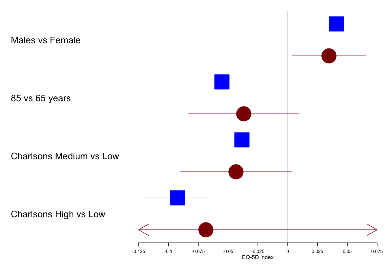
选择线型
forestplot(tabletext,
            fn.ci_norm = c(fpDrawNormalCI, fpDrawCircleCI),
            boxsize = .25, # We set the box size to better visualize the type
            line.margin = .1, # We need to add this to avoid crowding
            mean = cbind(HRQoL$Sweden[, "coef"], HRQoL$Denmark[, "coef"]),
            lower = cbind(HRQoL$Sweden[, "lower"], HRQoL$Denmark[, "lower"]),
            upper = cbind(HRQoL$Sweden[, "upper"], HRQoL$Denmark[, "upper"]),
            clip =c(-.125, 0.075),
            lty.ci = c(1, 2),
            col=fpColors(box=c("blue", "darkred")),
            xlab="EQ-5D index")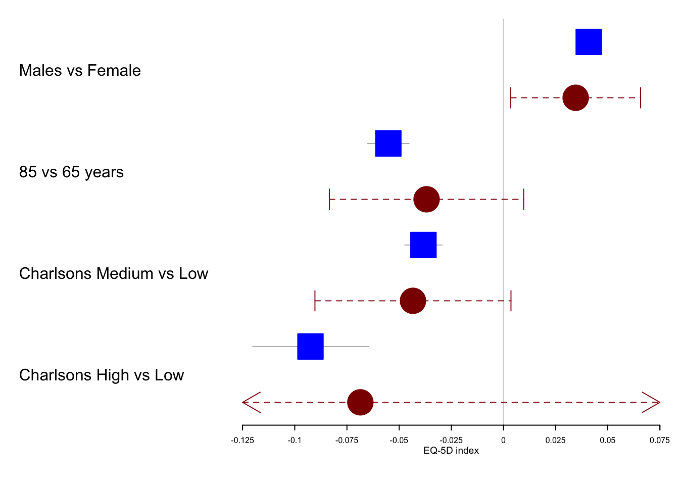
图例
添加一个基本图例:
forestplot(tabletext,
           legend = c("Sweden", "Denmark"),
           fn.ci_norm = c(fpDrawNormalCI, fpDrawCircleCI),
           boxsize = .25, # We set the box size to better visualize the type
           line.margin = .1, # We need to add this to avoid crowding
           mean = cbind(HRQoL$Sweden[, "coef"], HRQoL$Denmark[, "coef"]),
           lower = cbind(HRQoL$Sweden[, "lower"], HRQoL$Denmark[, "lower"]),
           upper = cbind(HRQoL$Sweden[, "upper"], HRQoL$Denmark[, "upper"]),
           clip =c(-.125, 0.075),
           col=fpColors(box=c("blue", "darkred")),
           xlab="EQ-5D index")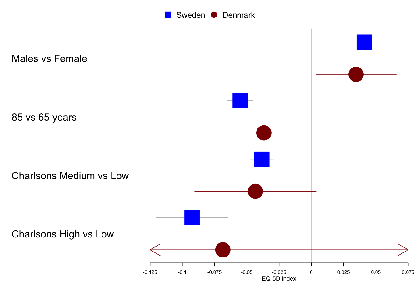
通过设定参数可以进一步自定义:
forestplot(tabletext,
           legend_args = fpLegend(pos = list(x=.85, y=0.25),
                                  gp=gpar(col="#CCCCCC", fill="#F9F9F9")),
           legend = c("Sweden", "Denmark"),
           fn.ci_norm = c(fpDrawNormalCI, fpDrawCircleCI),
           boxsize = .25, # We set the box size to better visualize the type
           line.margin = .1, # We need to add this to avoid crowding
           mean = cbind(HRQoL$Sweden[, "coef"], HRQoL$Denmark[, "coef"]),
           lower = cbind(HRQoL$Sweden[, "lower"], HRQoL$Denmark[, "lower"]),
           upper = cbind(HRQoL$Sweden[, "upper"], HRQoL$Denmark[, "upper"]),
           clip =c(-.125, 0.075),
           col=fpColors(box=c("blue", "darkred")),
           xlab="EQ-5D index")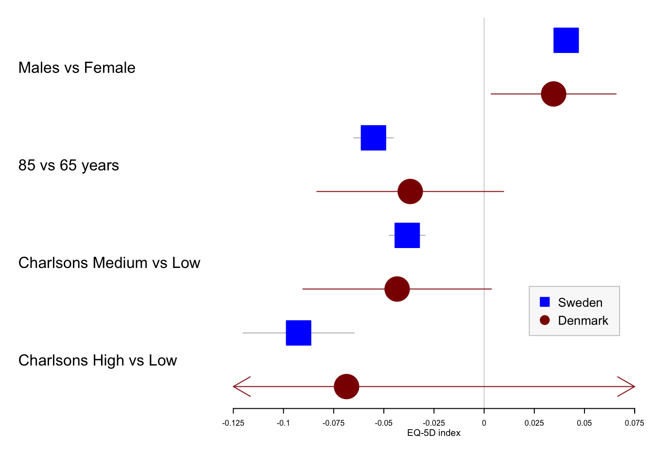
刻度和网格
我们可以手动设定想要的刻度
forestplot(tabletext,
           legend = c("Sweden", "Denmark"),
           fn.ci_norm = c(fpDrawNormalCI, fpDrawCircleCI),
           boxsize = .25, # We set the box size to better visualize the type
           line.margin = .1, # We need to add this to avoid crowding
           mean = cbind(HRQoL$Sweden[, "coef"], HRQoL$Denmark[, "coef"]),
           lower = cbind(HRQoL$Sweden[, "lower"], HRQoL$Denmark[, "lower"]),
           upper = cbind(HRQoL$Sweden[, "upper"], HRQoL$Denmark[, "upper"]),
           clip =c(-.125, 0.075),
           col=fpColors(box=c("blue", "darkred")),
           xticks = c(-.1, -0.05, 0, .05),
           xlab="EQ-5D index")
我们可以给想要的刻度加标签:
xticks <- seq(from = -.1, to = .05, by = 0.025)
xtlab <- rep(c(TRUE, FALSE), length.out = length(xticks))
attr(xticks, "labels") <- xtlab
forestplot(tabletext,
           legend = c("Sweden", "Denmark"),
           fn.ci_norm = c(fpDrawNormalCI, fpDrawCircleCI),
           boxsize = .25, # We set the box size to better visualize the type
           line.margin = .1, # We need to add this to avoid crowding
           mean = cbind(HRQoL$Sweden[, "coef"], HRQoL$Denmark[, "coef"]),
           lower = cbind(HRQoL$Sweden[, "lower"], HRQoL$Denmark[, "lower"]),
           upper = cbind(HRQoL$Sweden[, "upper"], HRQoL$Denmark[, "upper"]),
           clip =c(-.125, 0.075),
           col=fpColors(box=c("blue", "darkred")),
           xticks = xticks,
           xlab="EQ-5D index")
如果图形太高我们可能还需要增加辅助线以显示对应的刻度:
forestplot(tabletext,
           legend = c("Sweden", "Denmark"),
           fn.ci_norm = c(fpDrawNormalCI, fpDrawCircleCI),
           boxsize = .25, # We set the box size to better visualize the type
           line.margin = .1, # We need to add this to avoid crowding
           mean = cbind(HRQoL$Sweden[, "coef"], HRQoL$Denmark[, "coef"]),
           lower = cbind(HRQoL$Sweden[, "lower"], HRQoL$Denmark[, "lower"]),
           upper = cbind(HRQoL$Sweden[, "upper"], HRQoL$Denmark[, "upper"]),
           clip =c(-.125, 0.075),
           col=fpColors(box=c("blue", "darkred")),
           grid = TRUE,
           xticks = c(-.1, -0.05, 0, .05),
           xlab="EQ-5D index")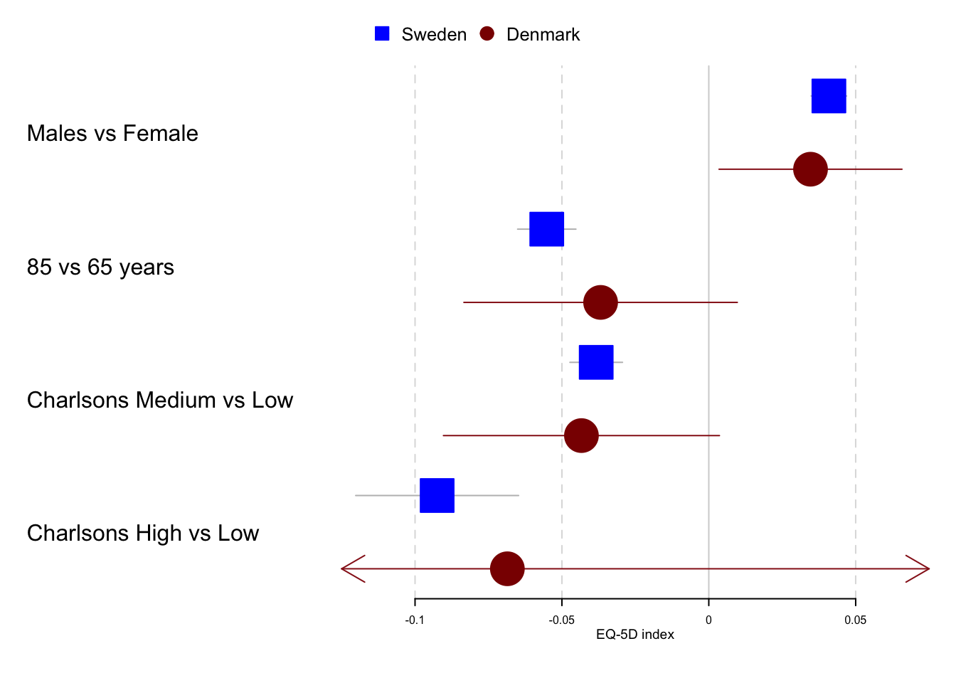
最后我们可以自定义想要的网格:
forestplot(tabletext,
           legend = c("Sweden", "Denmark"),
           fn.ci_norm = c(fpDrawNormalCI, fpDrawCircleCI),
           boxsize = .25, # We set the box size to better visualize the type
           line.margin = .1, # We need to add this to avoid crowding
           mean = cbind(HRQoL$Sweden[, "coef"], HRQoL$Denmark[, "coef"]),
           lower = cbind(HRQoL$Sweden[, "lower"], HRQoL$Denmark[, "lower"]),
           upper = cbind(HRQoL$Sweden[, "upper"], HRQoL$Denmark[, "upper"]),
           clip =c(-.125, 0.075),
           col=fpColors(box=c("blue", "darkred")),
           grid = structure(c(-.1, -.05, .05),
                            gp = gpar(lty = 2, col = "#CCCCFF")),
           xlab="EQ-5D index")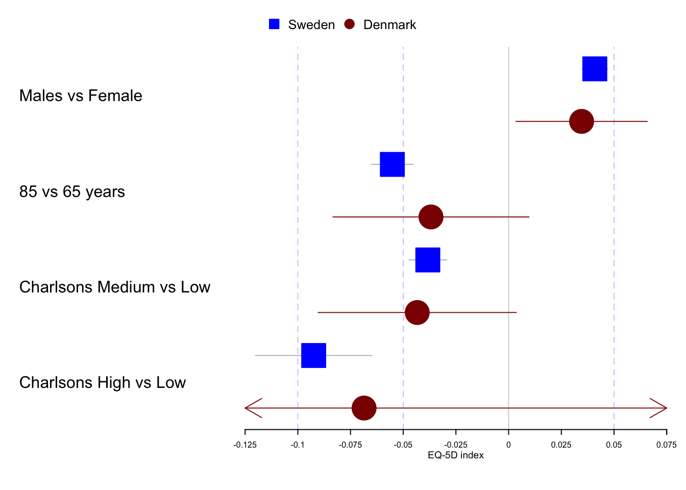
下面两种structure的书写方式是一致的:
grid_arg <- c(-.1, -.05, .05)
attr(grid_arg, "gp") <- gpar(lty = 2, col = "#CCCCFF")
identical(grid_arg,
          structure(c(-.1, -.05, .05),
                    gp = gpar(lty = 2, col = "#CCCCFF")))
#> [1] TRUE