6 Universal analysis
6.1 Association analysis and visualization
6.1.1 General numeric association
For general numeric association, you can use show_cor() function.
data("mtcars")
p1 <- show_cor(mtcars)
p2 <- show_cor(mtcars,
  x_vars = colnames(mtcars)[1:4],
  y_vars = colnames(mtcars)[5:8]
)
p3 <- show_cor(mtcars, vis_method = "circle", p_adj = "fdr")
p1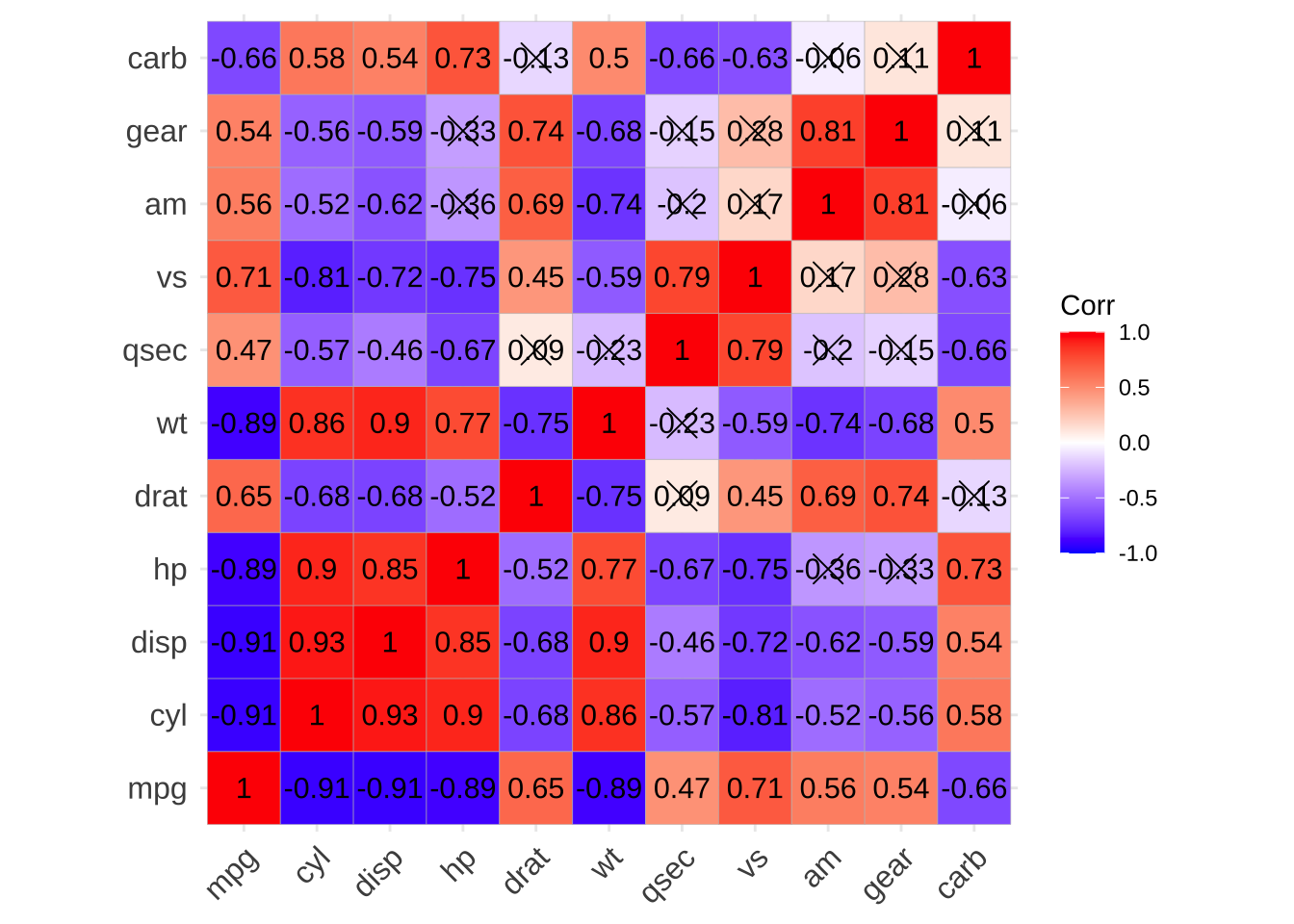
p1$cor
## $cor_mat
##        mpg   cyl  disp    hp  drat    wt  qsec    vs    am  gear  carb
## mpg   1.00 -0.91 -0.91 -0.89  0.65 -0.89  0.47  0.71  0.56  0.54 -0.66
## cyl  -0.91  1.00  0.93  0.90 -0.68  0.86 -0.57 -0.81 -0.52 -0.56  0.58
## disp -0.91  0.93  1.00  0.85 -0.68  0.90 -0.46 -0.72 -0.62 -0.59  0.54
## hp   -0.89  0.90  0.85  1.00 -0.52  0.77 -0.67 -0.75 -0.36 -0.33  0.73
## drat  0.65 -0.68 -0.68 -0.52  1.00 -0.75  0.09  0.45  0.69  0.74 -0.13
## wt   -0.89  0.86  0.90  0.77 -0.75  1.00 -0.23 -0.59 -0.74 -0.68  0.50
## qsec  0.47 -0.57 -0.46 -0.67  0.09 -0.23  1.00  0.79 -0.20 -0.15 -0.66
## vs    0.71 -0.81 -0.72 -0.75  0.45 -0.59  0.79  1.00  0.17  0.28 -0.63
## am    0.56 -0.52 -0.62 -0.36  0.69 -0.74 -0.20  0.17  1.00  0.81 -0.06
## gear  0.54 -0.56 -0.59 -0.33  0.74 -0.68 -0.15  0.28  0.81  1.00  0.11
## carb -0.66  0.58  0.54  0.73 -0.13  0.50 -0.66 -0.63 -0.06  0.11  1.00
##
## $p_mat
##               mpg          cyl         disp           hp         drat
## mpg  0.000000e+00 6.112687e-10 9.380327e-10 1.787835e-07 1.776240e-05
## cyl  6.112687e-10 0.000000e+00 1.802838e-12 3.477861e-09 8.244636e-06
## disp 9.380327e-10 1.802838e-12 0.000000e+00 7.142679e-08 5.282022e-06
## hp   1.787835e-07 3.477861e-09 7.142679e-08 0.000000e+00 9.988772e-03
## drat 1.776240e-05 8.244636e-06 5.282022e-06 9.988772e-03 0.000000e+00
## wt   1.293959e-10 1.217567e-07 1.222320e-11 4.145827e-05 4.784260e-06
## qsec 1.708199e-02 3.660533e-04 1.314404e-02 5.766253e-06 6.195826e-01
## vs   3.415937e-05 1.843018e-08 5.235012e-06 2.940896e-06 1.167553e-02
## am   2.850207e-04 2.151207e-03 3.662114e-04 1.798309e-01 4.726790e-06
## gear 5.400948e-03 4.173297e-03 9.635921e-04 4.930119e-01 8.360110e-06
## carb 1.084446e-03 1.942340e-03 2.526789e-02 7.827810e-07 6.211834e-01
##                wt         qsec           vs           am         gear
## mpg  1.293959e-10 1.708199e-02 3.415937e-05 2.850207e-04 5.400948e-03
## cyl  1.217567e-07 3.660533e-04 1.843018e-08 2.151207e-03 4.173297e-03
## disp 1.222320e-11 1.314404e-02 5.235012e-06 3.662114e-04 9.635921e-04
## hp   4.145827e-05 5.766253e-06 2.940896e-06 1.798309e-01 4.930119e-01
## drat 4.784260e-06 6.195826e-01 1.167553e-02 4.726790e-06 8.360110e-06
## wt   0.000000e+00 3.388683e-01 9.798492e-04 1.125440e-05 4.586601e-04
## qsec 3.388683e-01 0.000000e+00 1.029669e-06 2.056621e-01 2.425344e-01
## vs   9.798492e-04 1.029669e-06 0.000000e+00 3.570439e-01 2.579439e-01
## am   1.125440e-05 2.056621e-01 3.570439e-01 0.000000e+00 5.834043e-08
## gear 4.586601e-04 2.425344e-01 2.579439e-01 5.834043e-08 0.000000e+00
## carb 1.463861e-02 4.536949e-05 6.670496e-04 7.544526e-01 1.290291e-01
##              carb
## mpg  1.084446e-03
## cyl  1.942340e-03
## disp 2.526789e-02
## hp   7.827810e-07
## drat 6.211834e-01
## wt   1.463861e-02
## qsec 4.536949e-05
## vs   6.670496e-04
## am   7.544526e-01
## gear 1.290291e-01
## carb 0.000000e+00
p2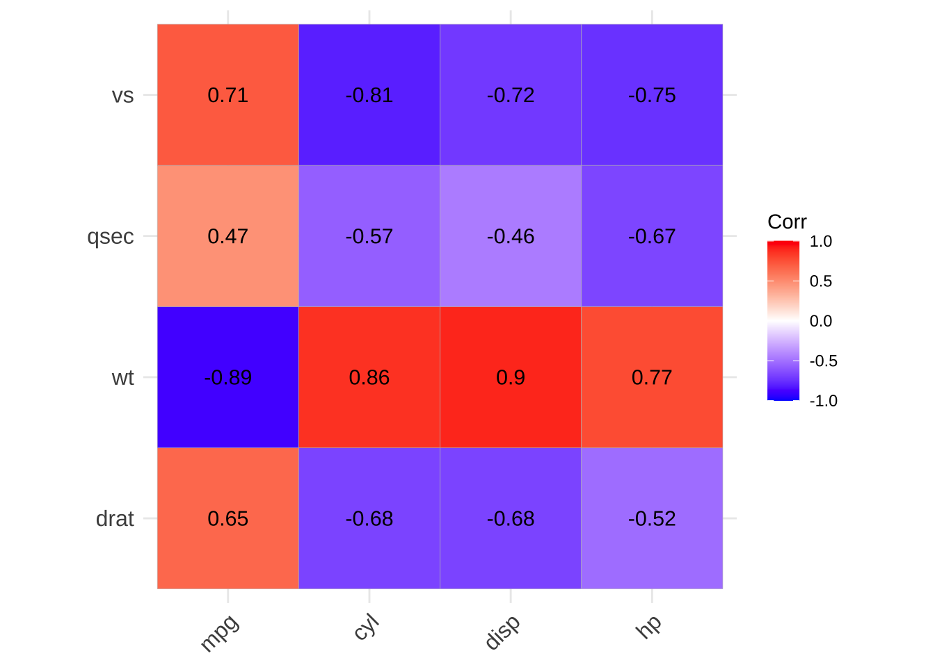
p3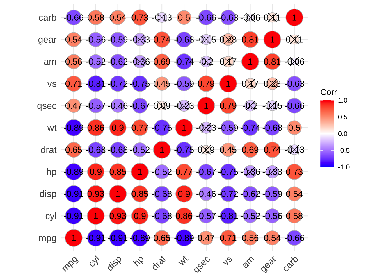
6.1.2 Comprehensive association
For comprehensive association analysis including both continuous and categorical variables, there are several functions available in sigminer:
Currently, I haven’t provided a proper example dataset for showing usage of all functions above (please read their documentation), here only the tidy dataset from our study (Wang et al. 2021) is given to show the plot function.
# The data is generated from Wang, Shixiang et al.
load(system.file("extdata", "asso_data.RData",
  package = "sigminer", mustWork = TRUE
))
p <- show_sig_feature_corrplot(tidy_data.seqz.feature, p_val = 0.05)
p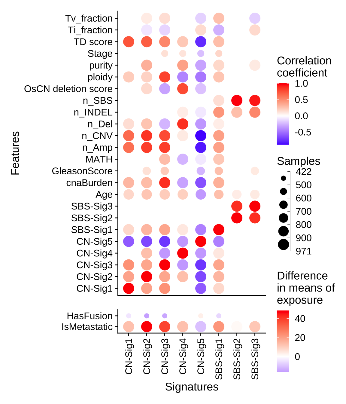
6.2 Group Analysis and Visualization
Group analysis is a common task in cancer study. Sigminer supports dividing samples into multiple groups and comparing genotype/phenotype feature measures.
6.2.1 Group Generation
There are multiple methods to generate groups, including ‘consensus’ (default, can be only used by result from sig_extract()), ‘k-means’ etc. After determining groups, sigminer will assign each group to a signature with maximum fraction. We may say a group is Sig_x enriched.
data("simulated_catalogs")
mt_sig <- sig_extract(t(simulated_catalogs$set1), n_sig = 10, nrun = 3)
## NMF algorithm: 'brunet'
## Multiple runs: 3
## Mode: sequential [foreach:doParallelMC]
##
Runs: |
Runs: |                                                  |   0%
Runs: |
Runs: |============                                      |  25%
Runs: |
Runs: |=========================                         |  50%
Runs: |
Runs: |======================================            |  75%
Runs: |
Runs: |==================================================| 100%
## System time:
##    user  system elapsed
##   5.108   0.031   5.148
mt_grps <- get_groups(mt_sig, method = "consensus", match_consensus = TRUE)
## ℹ [2022-08-29 12:00:04]: Started.
## ✔ [2022-08-29 12:00:04]: 'Signature' object detected.
## ℹ [2022-08-29 12:00:04]: Obtaining clusters from the hierarchical clustering of the consensus matrix...
## ℹ [2022-08-29 12:00:04]: Finding the dominant signature of each group...
## => Generating a table of group and dominant signature:
##
##      Sig1 Sig10 Sig2 Sig3 Sig4 Sig5 Sig7 Sig8 Sig9
##   1     0     2    0    2    0    0    0    0    0
##   10    1     0    0    1    0    4    0    0    0
##   2     0     0    1    0    0    0    0    0    0
##   3     1     0    0    0    0    0    0    0    0
##   4     1     0    1    0    2    0    0    0    0
##   5     0     0    0    0    0    0    0    1    0
##   6     1     0    1    0    0    0    2    0    0
##   7     0     0    0    0    0    0    0    0    3
##   8     0     0    1    4    0    0    0    0    0
##   9     1     0    0    0    0    0    0    0    0
## => Assigning a group to a signature with the maxium fraction (stored in 'map_table' attr)...
## ℹ [2022-08-29 12:00:05]: Summarizing...
##  group #1: 4 samples with Sig10 enriched.
##  group #10: 6 samples with Sig5 enriched.
##  group #2: 1 samples with Sig2 enriched.
##  group #3: 1 samples with Sig1 enriched.
##  group #4: 4 samples with Sig4 enriched.
##  group #5: 1 samples with Sig8 enriched.
##  group #6: 4 samples with Sig7 enriched.
##  group #7: 3 samples with Sig9 enriched.
##  group #8: 5 samples with Sig3 enriched.
##  group #9: 1 samples with Sig1 enriched.
## ! [2022-08-29 12:00:05]: The 'enrich_sig' column is set to dominant signature in one group, please check and make it consistent with biological meaning (correct it by hand if necessary).
## ℹ [2022-08-29 12:00:05]: 0.072 secs elapsed.
head(mt_grps)
##       sample group silhouette_width enrich_sig
## 1: Sample_14     1         6.67e-01      Sig10
## 2:  Sample_6     1         0.00e+00      Sig10
## 3:  Sample_2     1         1.00e+00      Sig10
## 4:  Sample_5     1         0.00e+00      Sig10
## 5: Sample_22     2         1.00e+00       Sig2
## 6: Sample_12     3         1.67e-16       Sig1
The returned sample orders match sample orders in clustered consensus matrix.
show_sig_consensusmap(mt_sig)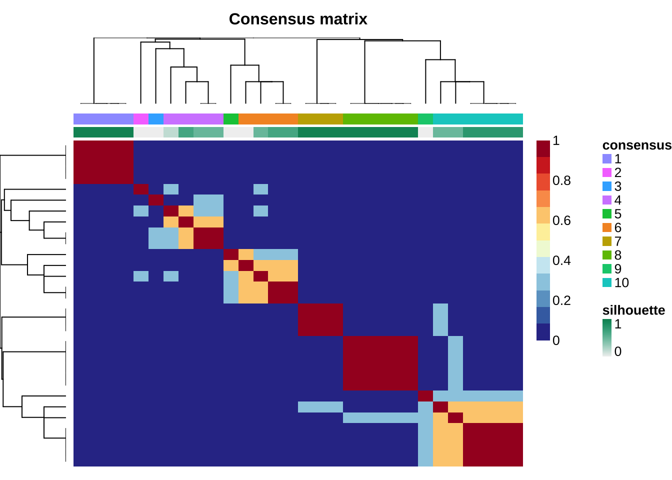
Sometimes, the mapping between groups and enriched signatures may not right. Users should check it and even correct it manually.
attr(mt_grps, "map_table")
##
##      Sig1 Sig10 Sig2 Sig3 Sig4 Sig5 Sig7 Sig8 Sig9
##   1     0     2    0    2    0    0    0    0    0
##   10    1     0    0    1    0    4    0    0    0
##   2     0     0    1    0    0    0    0    0    0
##   3     1     0    0    0    0    0    0    0    0
##   4     1     0    1    0    2    0    0    0    0
##   5     0     0    0    0    0    0    0    1    0
##   6     1     0    1    0    0    0    2    0    0
##   7     0     0    0    0    0    0    0    0    3
##   8     0     0    1    4    0    0    0    0    0
##   9     1     0    0    0    0    0    0    0    0
6.2.2 Group Comparison Analysis
load(system.file("extdata", "toy_copynumber_signature_by_W.RData",
package = "sigminer", mustWork = TRUE
))
# Assign samples to clusters
groups <- get_groups(sig, method = "k-means")
## ℹ [2022-08-29 12:00:05]: Started.
## ✔ [2022-08-29 12:00:05]: 'Signature' object detected.
## ℹ [2022-08-29 12:00:05]: Running k-means with 2 clusters...
## ℹ [2022-08-29 12:00:05]: Generating a table of group and signature contribution (stored in 'map_table' attr):
## Sig1 Sig2
## 1 0.2097559 0.7901116
## 2 0.8964984 0.1035016
## ℹ [2022-08-29 12:00:05]: Assigning a group to a signature with the maximum fraction...
## ℹ [2022-08-29 12:00:05]: Summarizing...
## group #1: 2 samples with Sig2 enriched.
## group #2: 8 samples with Sig1 enriched.
## ! [2022-08-29 12:00:05]: The 'enrich_sig' column is set to dominant signature in one group, please check and make it consistent with biological meaning (correct it by hand if necessary).
## ℹ [2022-08-29 12:00:05]: 0.031 secs elapsed.
set.seed(1234)
groups$prob <- rnorm(10)
groups$new_group <- sample(c("1", "2", "3", "4", NA), size = nrow(groups), replace = TRUE)
# Compare groups (filter NAs for categorical coloumns)
groups.cmp <- get_group_comparison(groups[, -1],
col_group = "group",
cols_to_compare = c("prob", "new_group"),
type = c("co", "ca"), verbose = TRUE
)
## Treat prob as continuous variable.
## Treat new_group as categorical variable.
# Compare groups (Set NAs of categorical columns to 'Rest')
groups.cmp2 <- get_group_comparison(groups[, -1],
col_group = "group",
cols_to_compare = c("prob", "new_group"),
type = c("co", "ca"), NAs = "Rest", verbose = TRUE
)
## Treat prob as continuous variable.
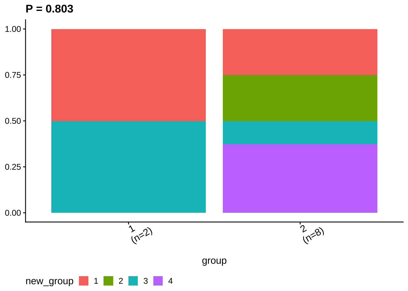
## Treat new_group as categorical variable.6.2.3 Group Visualization
ggcomp <- show_group_comparison(groups.cmp2)
ggcomp$co_comb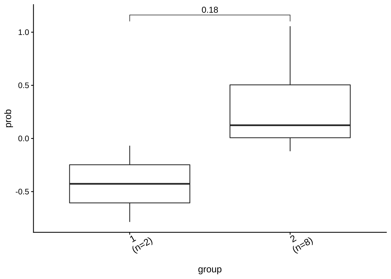
ggcomp$ca_comb