使用 sigminer 进行突变模式分析

王诗翔 · 2020-06-07

分类: r
标签: r sigminer mutational-signature

突变模式分析（Mutational Signature Analysis）已经逐步成为变异检测后一个通用分析，这篇文章简单介绍如何使用 sigminer 进行突变模式分析，以解决 2 大分析任务：

从头发现 Signatures
已知一些参考 Signatures，我们想要定量 Signature 的 Exposure（或称为 Activity）

支持 SBS、DBS、INDEL 以及 copynumber（研究中）。

安装

BiocManager::install("sigminer", dependencies = TRUE)

加载包

library(sigminer)
library(NMF)

数据输入

sigminer 的开发与 maftools 很有渊源，使用 MAF 对象作为数据的存储结构。如果你会使用 maftools 读入突变数据，那么就会使用 sigminer 读入突变数据，支持 data.frame 和 MAF 文件。

这里我们使用 maftools 内置数据集，maftools 其实本身也可以做 signature 分析（但不是它的核心）。

laml.maf <- system.file("extdata", "tcga_laml.maf.gz", package = "maftools", mustWork = TRUE)
laml <- read_maf(maf = laml.maf)
#> -Reading
#> -Validating
#> -Silent variants: 475 
#> -Summarizing
#> -Processing clinical data
#> --Missing clinical data
#> -Finished in 0.269s elapsed (0.245s cpu)
# 与 maftools::read.maf(maf = laml.maf) 结果是一样的
# read_maf 是对 read.maf 的封装

生成突变分类矩阵

使用 sig_tally() 对突变进行归类整理，针对 MAF 对象，支持设定 mode 为 ‘SBS’, ‘DBS’, ‘ID’ 以及 ‘ALL’。

mode 为 ’ALL` 时会尽量生成所有矩阵：

mats <- mt_tally <- sig_tally(
  laml,
  ref_genome = "BSgenome.Hsapiens.UCSC.hg19",
  useSyn = TRUE,
  mode = "ALL"
)

str(mats, max.level = 1)
#> List of 6
#>  $ SBS_6        : int [1:193, 1:6] 1 0 0 2 1 0 1 1 2 2 ...
#>   ..- attr(*, "dimnames")=List of 2
#>  $ SBS_96       : int [1:193, 1:96] 0 0 0 0 0 0 1 0 1 0 ...
#>   ..- attr(*, "dimnames")=List of 2
#>  $ SBS_1536     : int [1:193, 1:1536] 0 0 0 0 0 0 0 0 0 0 ...
#>   ..- attr(*, "dimnames")=List of 2
#>  $ ID_28        : int [1:193, 1:28] 0 0 0 0 0 0 0 0 0 0 ...
#>   ..- attr(*, "dimnames")=List of 2
#>  $ ID_83        : int [1:193, 1:83] 0 0 0 0 0 0 0 0 0 0 ...
#>   ..- attr(*, "dimnames")=List of 2
#>  $ APOBEC_scores:Classes 'data.table' and 'data.frame':  182 obs. of  44 variables:
#>   ..- attr(*, ".internal.selfref")=<externalptr> 
#>   ..- attr(*, "index")= int(0) 
#>   .. ..- attr(*, "__APOBEC_Enriched")= int [1:182] 106 147 5 6 8 9 10 11 12 13 ...

这个数据集没有双碱基替换，所以没有相应的矩阵。

mt_tally$SBS_96[1:5, 1:5]
#>              A[T>C]A C[T>C]A G[T>C]A T[T>C]A A[C>T]A
#> TCGA-AB-2802       0       0       0       0       0
#> TCGA-AB-2803       0       0       0       0       2
#> TCGA-AB-2804       0       0       0       0       2
#> TCGA-AB-2805       0       0       0       0       0
#> TCGA-AB-2806       0       0       0       0       0

针对整个数据集的分类就可以画图，Signatures 其实就是它的拆分。

show_catalogue(mt_tally$SBS_96 %>% t(), mode = "SBS", style = "cosmic")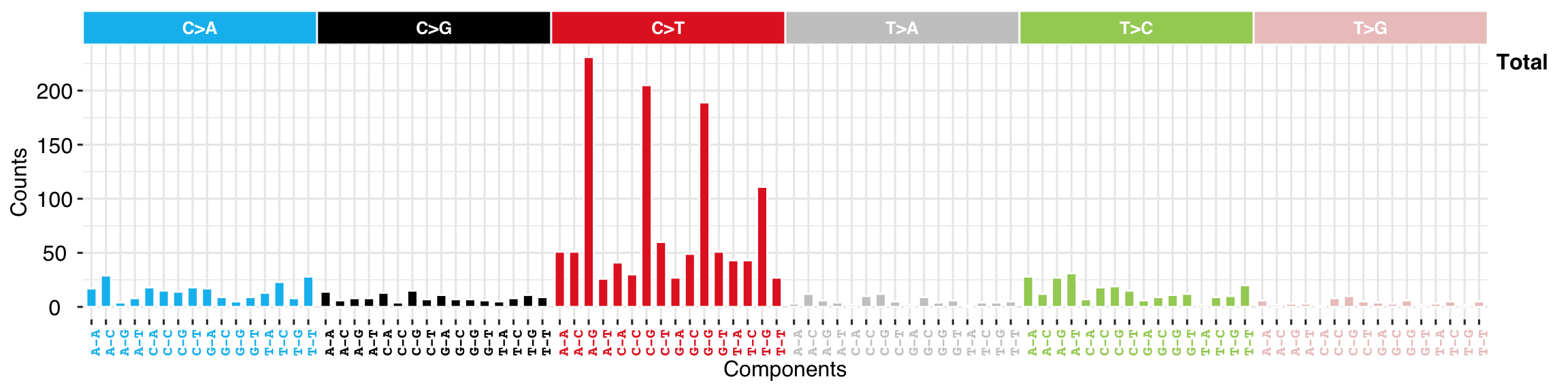

show_catalogue(mt_tally$SBS_6 %>% t(), mode = "SBS", style = "cosmic")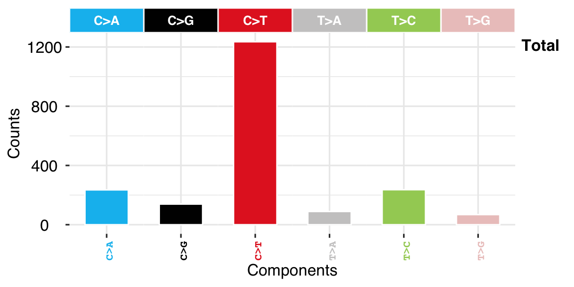

注意上面对矩阵进行了转置。

估计 Signature 数目

这一步实际上是多次运行 NMF，查看一些指标的变化，用于后续确定提取多少个 Signatures。

est <- sig_estimate(mt_tally$SBS_96, range = 2:5, nrun = 2, pConstant = 1e-9, verbose = TRUE)
#> Compute NMF rank= 2  ... + measures ... OK
#> Compute NMF rank= 3  ... + measures ... OK
#> Compute NMF rank= 4  ... + measures ... OK
#> Compute NMF rank= 5  ... + measures ... OK
#> Estimation of rank based on observed data.
#>   method   seed rng metric rank sparseness.basis sparseness.coef  rss  evar
#> 2 brunet random   1     KL    2            0.588           0.653 1924 0.411
#> 3 brunet random   1     KL    3            0.648           0.623 1875 0.426
#> 4 brunet random   1     KL    4            0.685           0.633 1802 0.448
#> 5 brunet random   1     KL    5            0.698           0.687 1723 0.472
#>   silhouette.coef silhouette.basis residuals niter   cpu cpu.all nrun
#> 2           1.000            1.000      2880  1040 0.467    4.39    2
#> 3           0.769            0.830      2718   800 0.438    4.17    2
#> 4           0.656            0.767      2543  1790 1.031    1.62    2
#> 5           0.609            0.712      2415  1750 1.139    4.93    2
#>   cophenetic dispersion silhouette.consensus
#> 2      0.888      0.576                0.712
#> 3      0.802      0.577                0.494
#> 4      0.784      0.655                0.473
#> 5      0.748      0.700                0.398

这里加入了一个 pConstant = 1e-9，是因为 NMF 包调用矩阵分解存在 bug，一个分类的和不能为 0。报错就加一个伪小数，不报错就可以不管。

show_sig_number_survey2(est$survey)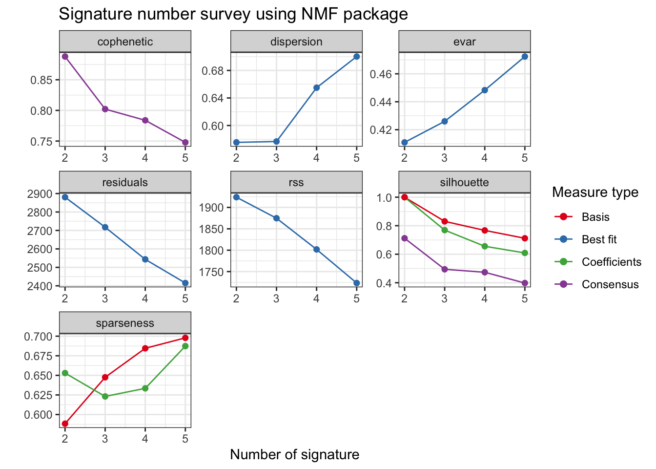

cophenetic 是一个主要指标，我们看到一直在下降。不过我们观测到残差，sparseness在往好的方向变化，这里可以选择 4 个试试（上面运行最好30-50次可以得到稳定结果）。

提取 signatures 和可视化

sigs <- sig_extract(mt_tally$SBS_96, n_sig = 4, nrun = 2, pConstant = 1e-9)

生成的是一个带 Signature 类信息的列表：

str(sigs, max.level = 1)
#> List of 6
#>  $ Signature     : num [1:96, 1:4] 1.90e-07 6.68e-08 1.07e-07 1.00 5.19e-09 ...
#>   ..- attr(*, "dimnames")=List of 2
#>  $ Signature.norm: num [1:96, 1:4] 3.38e-10 1.19e-10 1.90e-10 1.78e-03 9.23e-12 ...
#>   ..- attr(*, "dimnames")=List of 2
#>  $ Exposure      : num [1:4, 1:193] 2.02 3.69 4.05 2.43e-01 1.00e-13 ...
#>   ..- attr(*, "dimnames")=List of 2
#>  $ Exposure.norm : num [1:4, 1:193] 2.02e-01 3.69e-01 4.05e-01 2.43e-02 7.14e-15 ...
#>   ..- attr(*, "dimnames")=List of 2
#>  $ K             : int 4
#>  $ Raw           :List of 3
#>  - attr(*, "class")= chr "Signature"
#>  - attr(*, "nrun")= num 2
#>  - attr(*, "method")= chr "brunet"
#>  - attr(*, "pConstant")= num 1e-09
#>  - attr(*, "seed")= num 123456
#>  - attr(*, "call_method")= chr "NMF"

很多信息存在里面，用户可以自己提取自己感兴趣的信息。sigminer 也有很多函数专门用户提取一些信息、可视化等等。

我们先看一个最常见的突变模式图谱：

p <- show_sig_profile(sigs, mode = "SBS", style = "cosmic")
p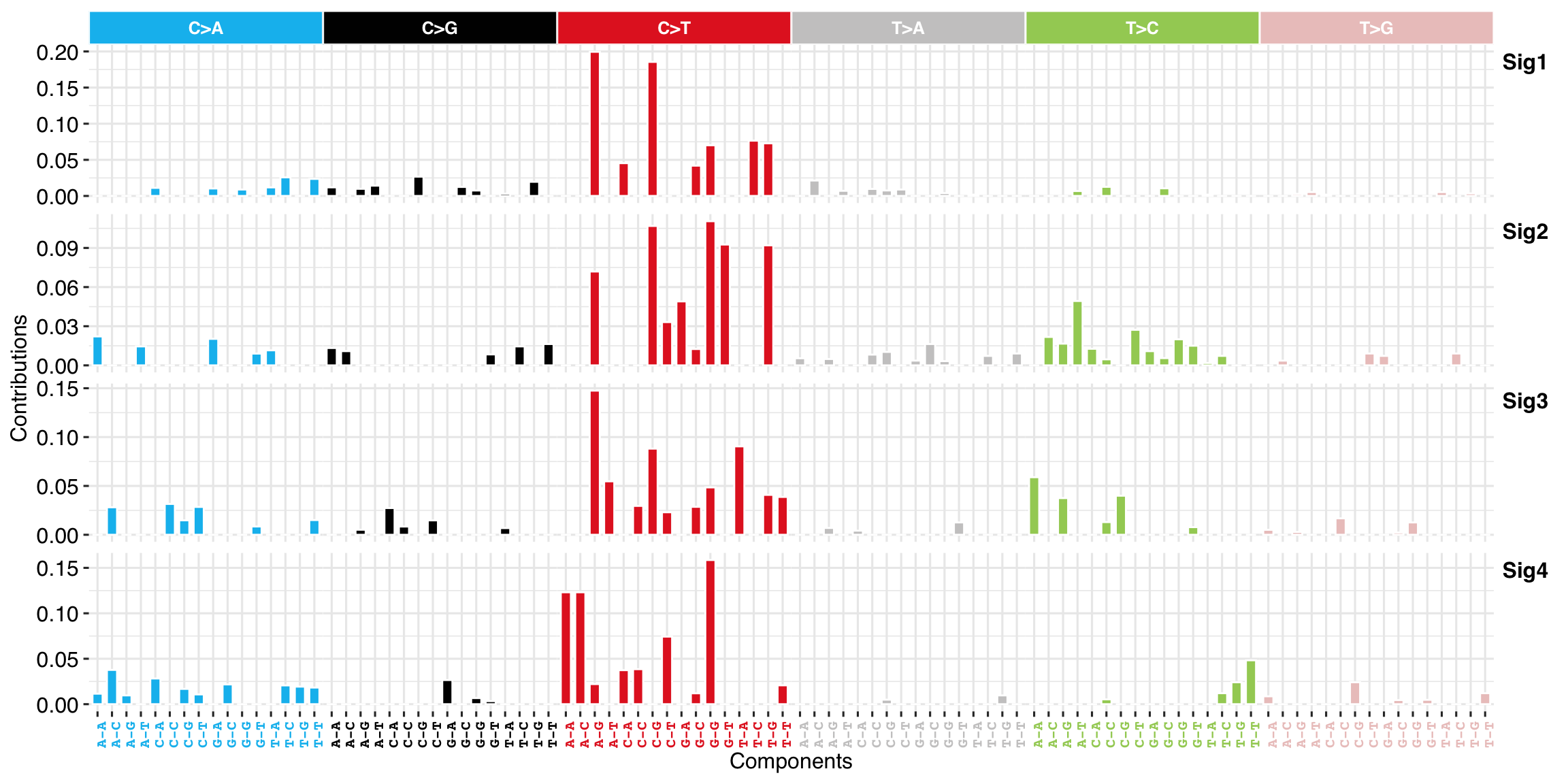

接着可以计算下它与 COSMIC signatures 的相似性，评估病因，对于 SBS 有 2 个 COSMIC 数据库版本 legacy（30 个，目前最常用的）与 SBS v3。

get_sig_similarity(sigs, sig_db = "legacy")
#> -Comparing against COSMIC signatures
#> ------------------------------------
#> --Found Sig1 most similar to COSMIC_1
#>    Aetiology: spontaneous deamination of 5-methylcytosine [similarity: 0.89]
#> --Found Sig2 most similar to COSMIC_6
#>    Aetiology: defective DNA mismatch repair [similarity: 0.797]
#> --Found Sig3 most similar to COSMIC_1
#>    Aetiology: spontaneous deamination of 5-methylcytosine [similarity: 0.8]
#> --Found Sig4 most similar to COSMIC_15
#>    Aetiology: defective DNA mismatch repair [similarity: 0.535]
#> ------------------------------------
#> Return result invisiblely.

sim <- get_sig_similarity(sigs, sig_db = "SBS")
#> -Comparing against COSMIC signatures
#> ------------------------------------
#> --Found Sig1 most similar to SBS1
#>    Aetiology: spontaneous or enzymatic deamination of 5-methylcytosine [similarity: 0.878]
#> --Found Sig2 most similar to SBS6
#>    Aetiology: defective DNA mismatch repair [similarity: 0.803]
#> --Found Sig3 most similar to SBS1
#>    Aetiology: spontaneous or enzymatic deamination of 5-methylcytosine [similarity: 0.737]
#> --Found Sig4 most similar to SBS15
#>    Aetiology: Defective DNA mismatch repair [similarity: 0.567]
#> ------------------------------------
#> Return result invisiblely.

add_labels(p, x = 0.72, y = 0.25, y_end = 0.9, labels = sim, n_label = 4)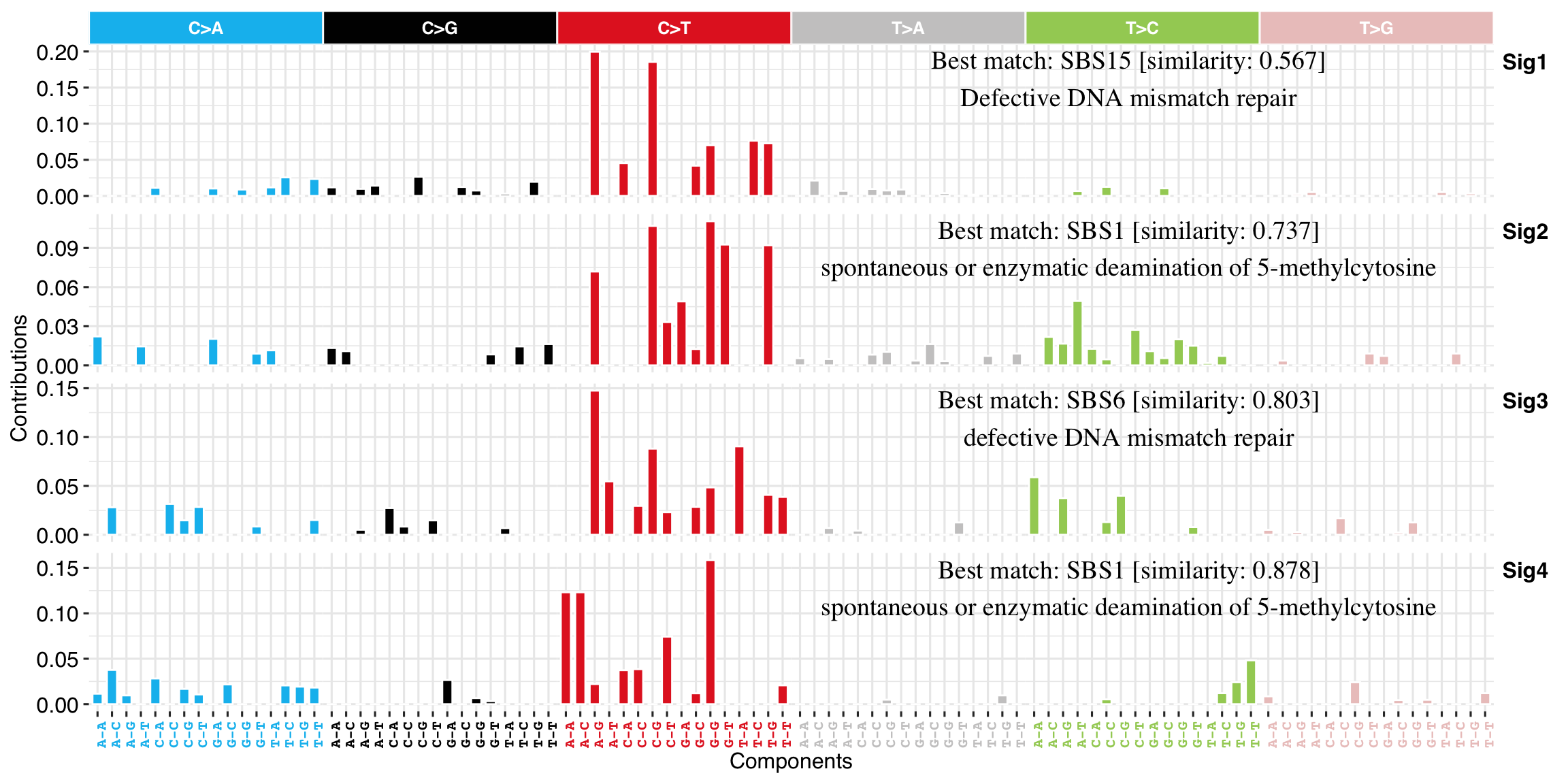

这里的坐标位置需要自己细调一下。

自动提取 signatures

SignatureAnalyzer 提供的变异 NMF 提供了自动提取 Sigantures 的功能，无需要自己判断提取的 signature 数目，这个可以通过 sig_auto_extract() 实现。该算法会倾向生成更加稀疏（相互之间不一致）的 signatures，因此偏向于生成更多的 signatures。从我多年研究 signatures 的经验来看，它对于单点突变还是非常友好的。

sigs2 <- sig_auto_extract(mt_tally$SBS_96, nrun = 2)
#> Warning: [ONE-TIME WARNING] Forked processing ('multicore') is disabled
#> in future (>= 1.13.0) when running R from RStudio, because it is
#> considered unstable. Because of this, plan("multicore") will fall
#> back to plan("sequential"), and plan("multiprocess") will fall back to
#> plan("multisession") - not plan("multicore") as in the past. For more details,
#> how to control forked processing or not, and how to silence this warning in
#> future R sessions, see ?future::supportsMulticore
#> 
#> Attaching package: 'purrr'
#> The following objects are masked from 'package:foreach':
#> 
#>     accumulate, when
#> The following object is masked from 'package:XVector':
#> 
#>     compact
#> The following object is masked from 'package:GenomicRanges':
#> 
#>     reduce
#> The following object is masked from 'package:IRanges':
#> 
#>     reduce
#> Select Run 1, which K = 2 as best solution.

画图方式是完全一样的。

p <- show_sig_profile(sigs2, mode = "SBS", style = "cosmic")
p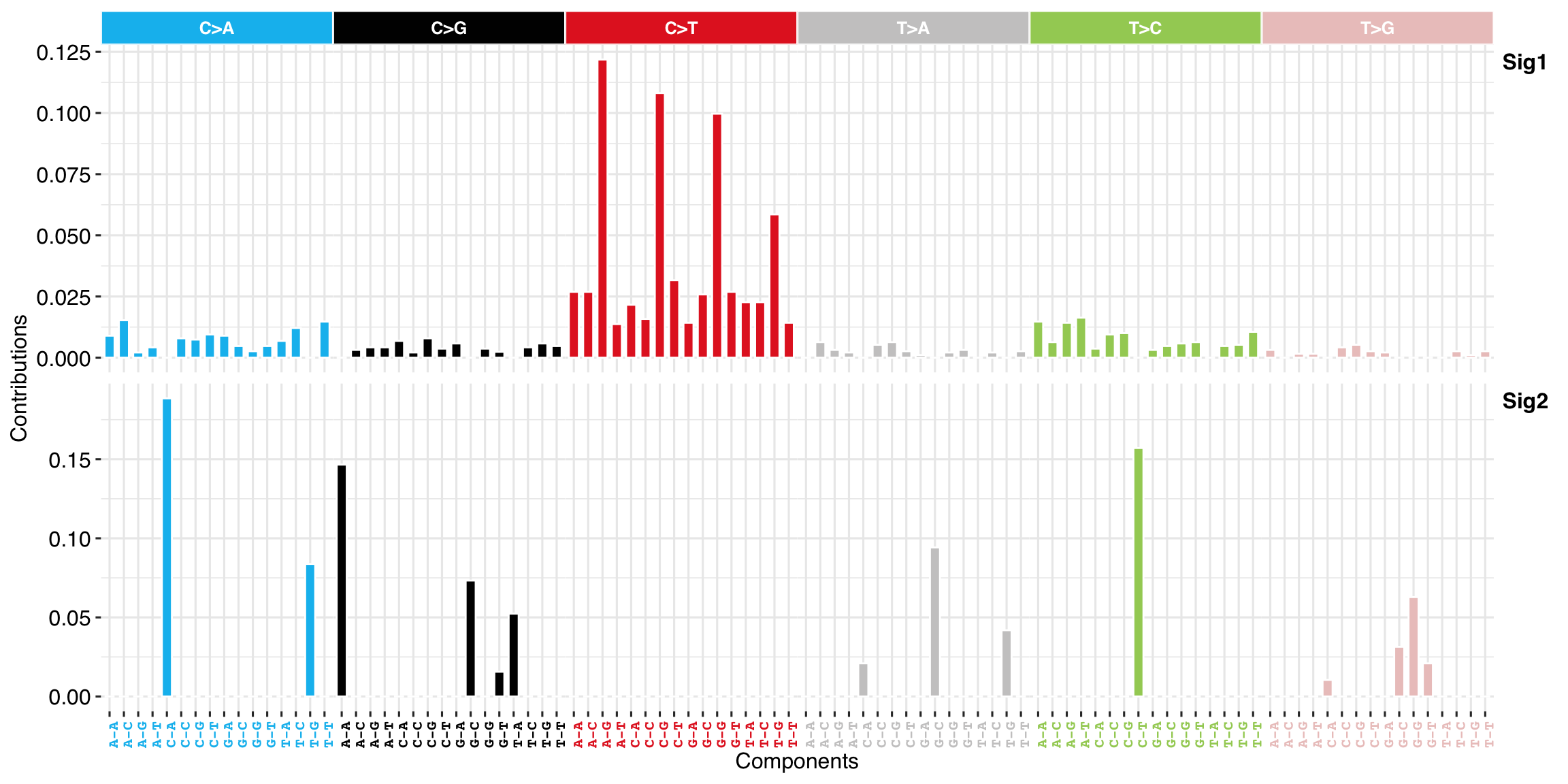

虽然上面都是粗略的分析，但这种方法感觉更好。

实际研究时选择哪种方法都需要根据数据还自己的需要决定，也可以比较两者的结果。

Signature 活动图谱

sigminer 提供绝对和相对两种 Signature 活动度值。

get_sig_exposure(sigs2) %>% head()
#>          sample  Sig1  Sig2
#> 1: TCGA-AB-2802  9.52 0.000
#> 2: TCGA-AB-2803 13.09 0.000
#> 3: TCGA-AB-2804  5.82 0.444
#> 4: TCGA-AB-2805 13.09 0.000
#> 5: TCGA-AB-2806 13.96 0.000
#> 6: TCGA-AB-2807 23.95 0.000
get_sig_exposure(sigs2, type = "relative") %>% head()
#> Filtering the samples with no signature exposure:
#> TCGA-AB-2823 TCGA-AB-2834 TCGA-AB-2840 TCGA-AB-2848 TCGA-AB-2909 TCGA-AB-2942
#>          sample  Sig1   Sig2
#> 1: TCGA-AB-2802 1.000 0.0000
#> 2: TCGA-AB-2803 1.000 0.0000
#> 3: TCGA-AB-2804 0.929 0.0709
#> 4: TCGA-AB-2805 1.000 0.0000
#> 5: TCGA-AB-2806 1.000 0.0000
#> 6: TCGA-AB-2807 1.000 0.0000

画图直接把对象扔进去就可以了。

show_sig_exposure(sigs, rm_space = TRUE, style = "cosmic")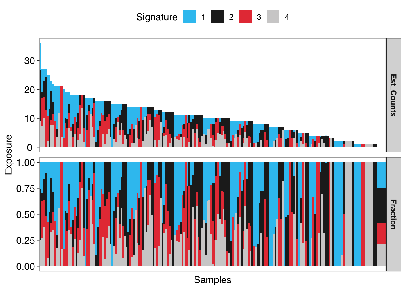

根据已知的 Signatures 提取活动度

这个比较有名的软件就是 deconstructSigs 了。sigminer 也支持了这个功能，而且能够使用目前 cosmic 的所有图谱，也可以使用自己从头发现的 signatures。函数就一个 sig_fit()。

我们试着处理 5 个样本（支持单样本），使用 COSMIC v2 30 个 signatures 作为参考。

examp_fit <- sig_fit(mt_tally$SBS_96[1:5, ] %>% t(), sig_index = "ALL", sig_db = "legacy")
head(examp_fit)
#>          TCGA-AB-2802 TCGA-AB-2803 TCGA-AB-2804 TCGA-AB-2805 TCGA-AB-2806
#> COSMIC_1        3.129        10.00            7         13.6         10.8
#> COSMIC_2        0.895         0.00            0          0.0          0.0
#> COSMIC_3        0.000         0.00            0          0.0          0.0
#> COSMIC_4        0.000         1.72            0          0.0          0.0
#> COSMIC_5        0.000         0.00            0          0.0          0.0
#> COSMIC_6        1.088         0.00            0          0.0          0.0

画图也很简单：

show_sig_fit(examp_fit, palette = NULL) + ggpubr::rotate_x_text()
#> ℹ [2020-08-09 13:35:51]: Started.
#> ℹ [2020-08-09 13:35:51]: Checking input format.
#> ✓ [2020-08-09 13:35:51]: Checked.
#> ℹ [2020-08-09 13:35:51]: Checking filters.
#> ℹ [2020-08-09 13:35:51]: Checked.
#> ℹ [2020-08-09 13:35:51]: Plotting.
#> ℹ [2020-08-09 13:35:51]: 0.054 secs elapsed.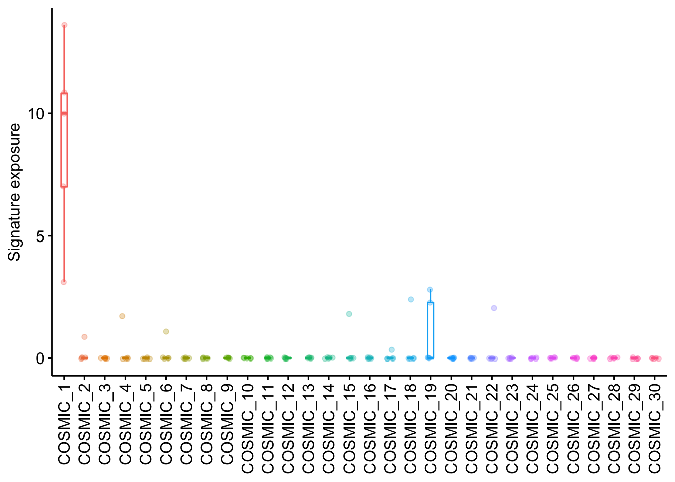

如果设置散点图，可以把单样本结果画出来。

show_sig_fit(examp_fit,
  palette = NULL, plot_fun = "scatter",
  signatures = paste0("COSMIC_", c(1, 2, 4, 6, 19))
) + ggpubr::rotate_x_text()
#> ℹ [2020-08-09 13:35:52]: Started.
#> ℹ [2020-08-09 13:35:52]: Checking input format.
#> ✓ [2020-08-09 13:35:52]: Checked.
#> ℹ [2020-08-09 13:35:52]: Checking filters.
#> ℹ [2020-08-09 13:35:52]: Checked.
#> ℹ [2020-08-09 13:35:52]: Plotting.
#> ! [2020-08-09 13:35:52]: When plot_fun='scatter', setting legend='top' is recommended.
#> ℹ [2020-08-09 13:35:52]: 0.042 secs elapsed.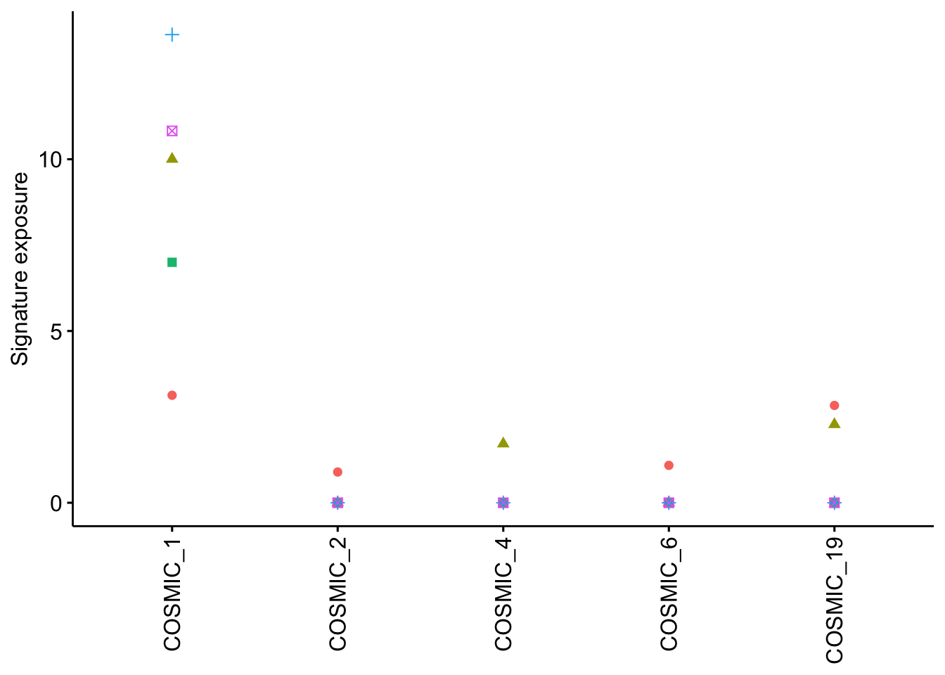

上面展示了最核心的分析和可视化功能，sigminer 还支持很多功能，我就不再详述了。用户可以阅读官方文档 https://shixiangwang.github.io/sigminer-doc/ 进一步学习，后续我会根据研究情况进一步开发。当然，读者完全可以基于上面分析的结果值进行各种个性化分析。