Chapter 9 Association Analysis and Visualization
9.1 General numeric association
For general numeric association, you can use show_cor() function.
data("mtcars")
p1 <- show_cor(mtcars)
p2 <- show_cor(mtcars,
  x_vars = colnames(mtcars)[1:4],
  y_vars = colnames(mtcars)[5:8]
)
p3 <- show_cor(mtcars, vis_method = "circle", p_adj = "fdr")
p1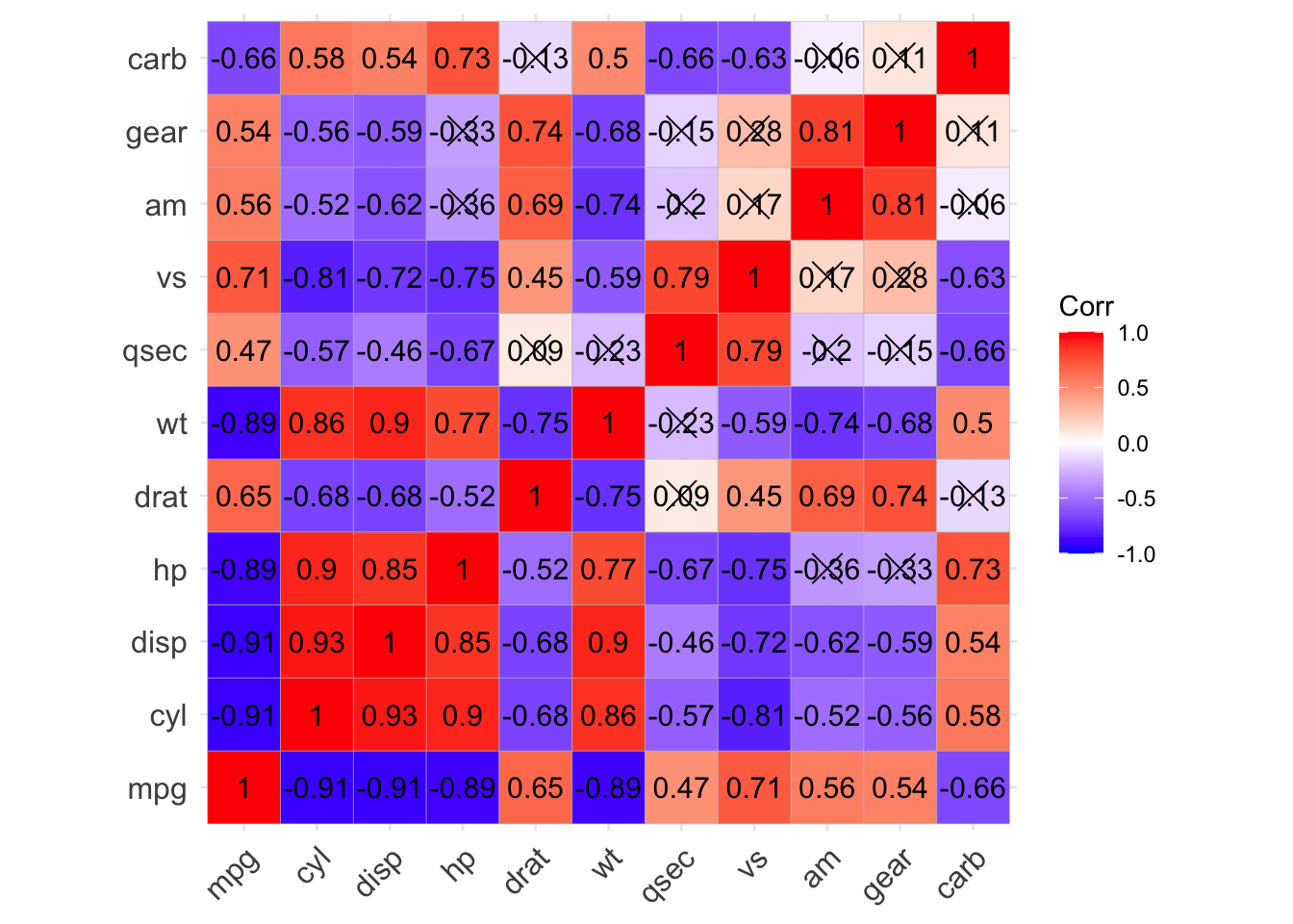
p1$cor
#> $cor_mat
#>        mpg   cyl  disp    hp  drat    wt  qsec    vs    am  gear  carb
#> mpg   1.00 -0.91 -0.91 -0.89  0.65 -0.89  0.47  0.71  0.56  0.54 -0.66
#> cyl  -0.91  1.00  0.93  0.90 -0.68  0.86 -0.57 -0.81 -0.52 -0.56  0.58
#> disp -0.91  0.93  1.00  0.85 -0.68  0.90 -0.46 -0.72 -0.62 -0.59  0.54
#> hp   -0.89  0.90  0.85  1.00 -0.52  0.77 -0.67 -0.75 -0.36 -0.33  0.73
#> drat  0.65 -0.68 -0.68 -0.52  1.00 -0.75  0.09  0.45  0.69  0.74 -0.13
#> wt   -0.89  0.86  0.90  0.77 -0.75  1.00 -0.23 -0.59 -0.74 -0.68  0.50
#> qsec  0.47 -0.57 -0.46 -0.67  0.09 -0.23  1.00  0.79 -0.20 -0.15 -0.66
#> vs    0.71 -0.81 -0.72 -0.75  0.45 -0.59  0.79  1.00  0.17  0.28 -0.63
#> am    0.56 -0.52 -0.62 -0.36  0.69 -0.74 -0.20  0.17  1.00  0.81 -0.06
#> gear  0.54 -0.56 -0.59 -0.33  0.74 -0.68 -0.15  0.28  0.81  1.00  0.11
#> carb -0.66  0.58  0.54  0.73 -0.13  0.50 -0.66 -0.63 -0.06  0.11  1.00
#>
#> $p_mat
#>               mpg          cyl         disp           hp         drat           wt
#> mpg  0.000000e+00 6.112687e-10 9.380327e-10 1.787835e-07 1.776240e-05 1.293959e-10
#> cyl  6.112687e-10 0.000000e+00 1.802838e-12 3.477861e-09 8.244636e-06 1.217567e-07
#> disp 9.380327e-10 1.802838e-12 0.000000e+00 7.142679e-08 5.282022e-06 1.222320e-11
#> hp   1.787835e-07 3.477861e-09 7.142679e-08 0.000000e+00 9.988772e-03 4.145827e-05
#> drat 1.776240e-05 8.244636e-06 5.282022e-06 9.988772e-03 0.000000e+00 4.784260e-06
#> wt   1.293959e-10 1.217567e-07 1.222320e-11 4.145827e-05 4.784260e-06 0.000000e+00
#> qsec 1.708199e-02 3.660533e-04 1.314404e-02 5.766253e-06 6.195826e-01 3.388683e-01
#> vs   3.415937e-05 1.843018e-08 5.235012e-06 2.940896e-06 1.167553e-02 9.798492e-04
#> am   2.850207e-04 2.151207e-03 3.662114e-04 1.798309e-01 4.726790e-06 1.125440e-05
#> gear 5.400948e-03 4.173297e-03 9.635921e-04 4.930119e-01 8.360110e-06 4.586601e-04
#> carb 1.084446e-03 1.942340e-03 2.526789e-02 7.827810e-07 6.211834e-01 1.463861e-02
#>              qsec           vs           am         gear         carb
#> mpg  1.708199e-02 3.415937e-05 2.850207e-04 5.400948e-03 1.084446e-03
#> cyl  3.660533e-04 1.843018e-08 2.151207e-03 4.173297e-03 1.942340e-03
#> disp 1.314404e-02 5.235012e-06 3.662114e-04 9.635921e-04 2.526789e-02
#> hp   5.766253e-06 2.940896e-06 1.798309e-01 4.930119e-01 7.827810e-07
#> drat 6.195826e-01 1.167553e-02 4.726790e-06 8.360110e-06 6.211834e-01
#> wt   3.388683e-01 9.798492e-04 1.125440e-05 4.586601e-04 1.463861e-02
#> qsec 0.000000e+00 1.029669e-06 2.056621e-01 2.425344e-01 4.536949e-05
#> vs   1.029669e-06 0.000000e+00 3.570439e-01 2.579439e-01 6.670496e-04
#> am   2.056621e-01 3.570439e-01 0.000000e+00 5.834043e-08 7.544526e-01
#> gear 2.425344e-01 2.579439e-01 5.834043e-08 0.000000e+00 1.290291e-01
#> carb 4.536949e-05 6.670496e-04 7.544526e-01 1.290291e-01 0.000000e+00
p2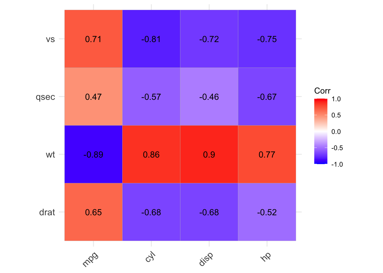
p3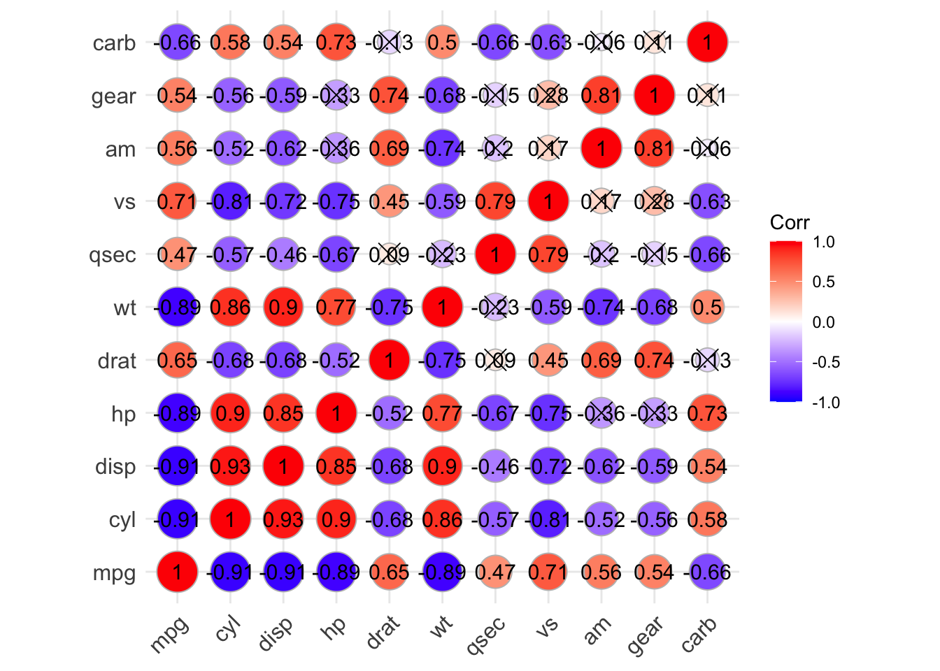
9.2 Comprehensive association
For comprehensive association analysis including both continuous and categorical variables, there are several functions available in sigminer:
get_sig_feature_association().get_tidy_association().show_sig_feature_corrplot().
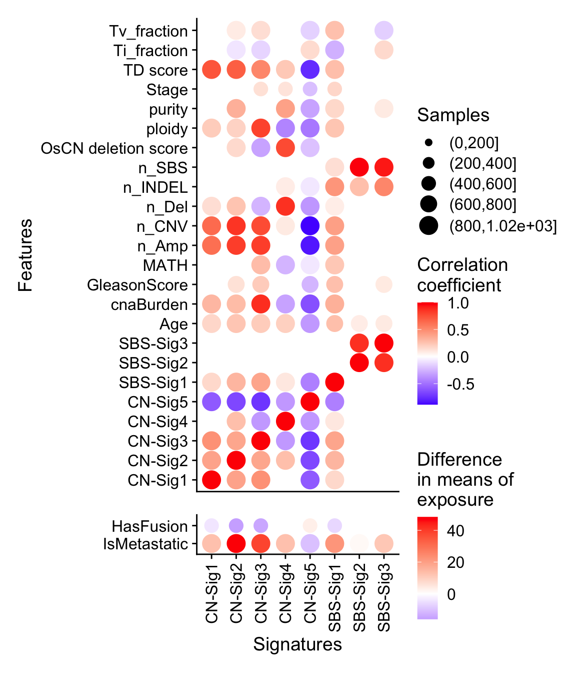
Currently, I haven’t provided a proper example dataset for showing usage of all functions above (please read their documentation), here only the tidy dataset from our study (Wang et al. 2020) is given to show the plot function.
# The data is generated from Wang, Shixiang et al.
load(system.file("extdata", "asso_data.RData",
  package = "sigminer", mustWork = TRUE
))

p <- show_sig_feature_corrplot(tidy_data.seqz.feature, p_val = 0.05)
#> Warning: Using size for a discrete variable is not advised.

#> Warning: Using size for a discrete variable is not advised.
p