Chapter 8 Signature Object
Signature is a core object in sigminer, it stores signatures and their exposures. Here we show how to plot signature profile and exposure profile. The result plots are basically ggplot based, so they can be further edited by your custom operations with ggplot grammar.
8.1 Signature Profile
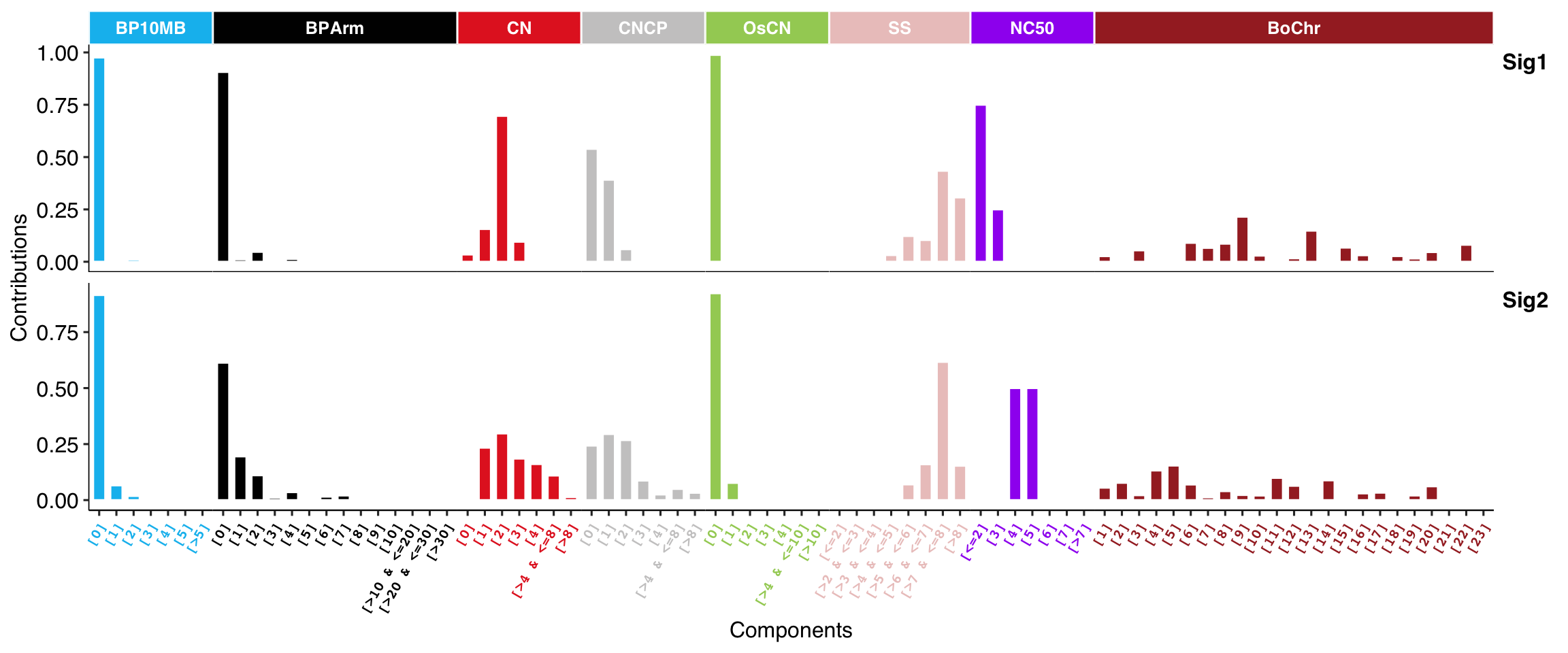
A signature is composed of distinct component patterns. They can be shown by show_sig_profile(). Of note, for different types of signature, the bar heights may have different meanings.
- SBS signatures are displayed based on the observed component frequency of the human genome, i.e., representing the relative proportions of mutations generated by each signature based on the actual trinucleotide frequencies of the reference human genome.
- Similar to SBS signatures, copy number signatures are displayed based on the observed component frequency of the human genome. Of note, considering the count process of each feature is relatively independent, the profile is row normalized by each feature, unlike Macintyre et al. (2018) did column normalization (this method is easy to mislead readers), so the bar height can be compared within/between features.
8.1.1 SBS Signature profile
show_sig_profile(mt_sig, mode = "SBS", paint_axis_text = FALSE, x_label_angle = 90)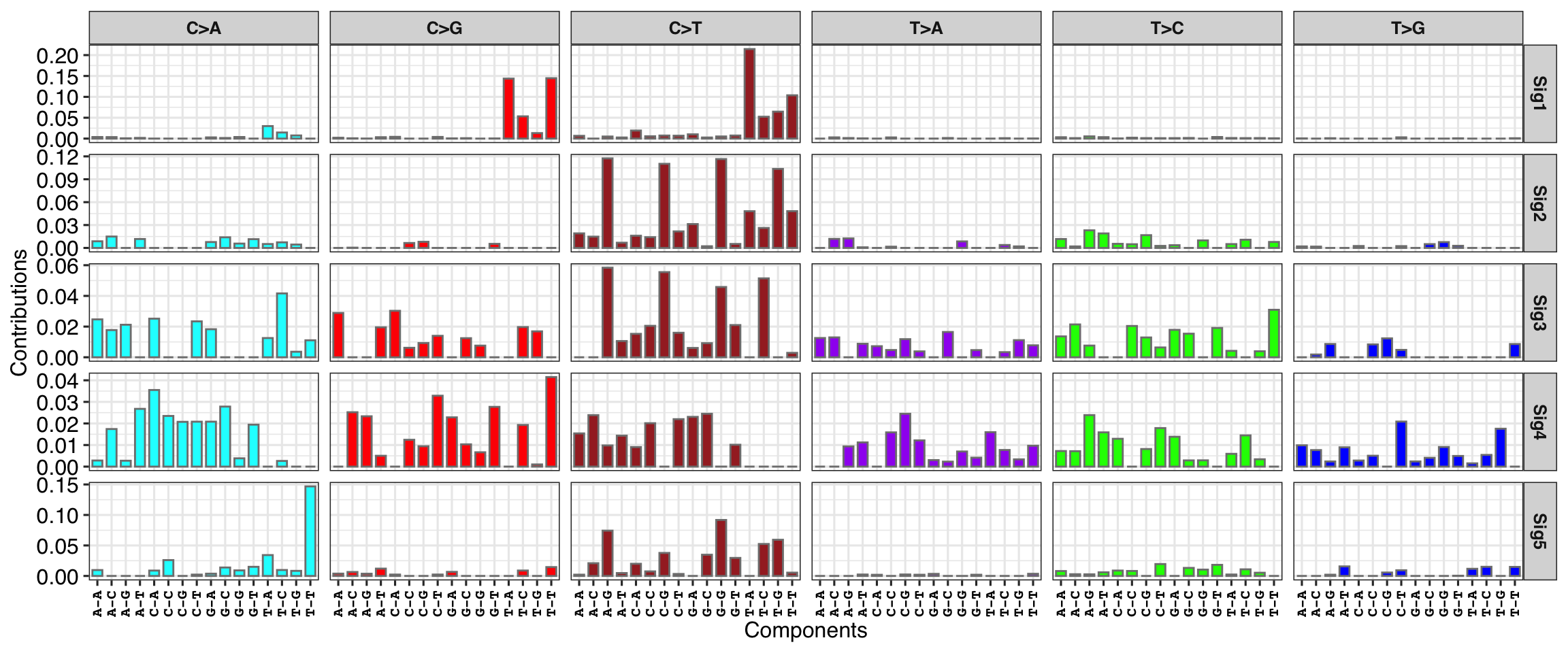
show_sig_profile(mt_sig, mode = "SBS", style = "cosmic", x_label_angle = 90)
#> Bioconductor version 3.12 (BiocManager 1.30.12), ?BiocManager::install for help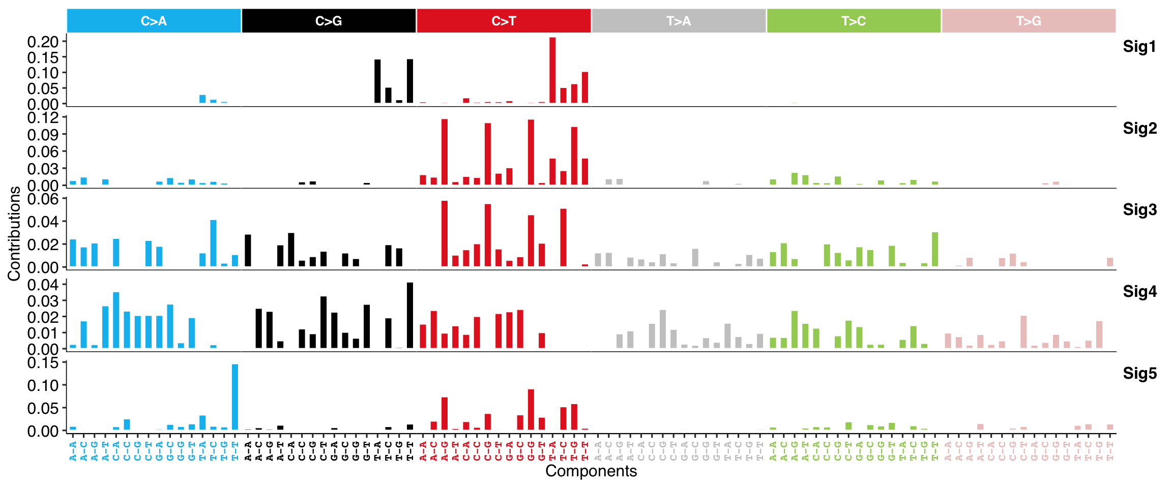
8.1.2 Copy Number Signature Porfile
For copy number signatures from tally method “W,” you have to specify the normalize option as “feature,” so the bar heights can be more clearly compared.
show_sig_profile(sig_w,
  mode = "copynumber",
  normalize = "feature",
  method = "W",
  style = "cosmic"
)
8.1.3 COSMIC Signature Profile
Users can show profile of COSMIC signatures by show_cosmic_sig_profile().
To see valid signature numbers, run
show_cosmic_sig_profile(sig_db = "legacy")
#>
#> Valid index for db 'legacy':
#> 1 2 3 4 5 6 7 8 9 10 11 12 13 14 15 16 17 18 19 20 21 22 23 24 25 26 27 28 29 30
‘legacy’ is for COSMIC v2.
show_cosmic_sig_profile(sig_db = "SBS")
#>
#> Valid index for db 'SBS':
#> 1 2 3 4 5 6 7a 7b 7c 7d 8 9 10a 10b 11 12 13 14 15 16 17a 17b 18 19 20 21 22 23 24 25 26 27 28 29 30 31 32 33 34 35 36 37 38 39 40 41 42 43 44 45 46 47 48 49 50 51 52 53 54 55 56 57 58 59 60 84 85 86 87 88 89 90
To show the plot, specify signature shortnames to sig_index option.
show_cosmic_sig_profile(sig_index = c(1, 5, 6), style = "cosmic")
#>
#> Valid index for db 'legacy':
#> 1 2 3 4 5 6 7 8 9 10 11 12 13 14 15 16 17 18 19 20 21 22 23 24 25 26 27 28 29 30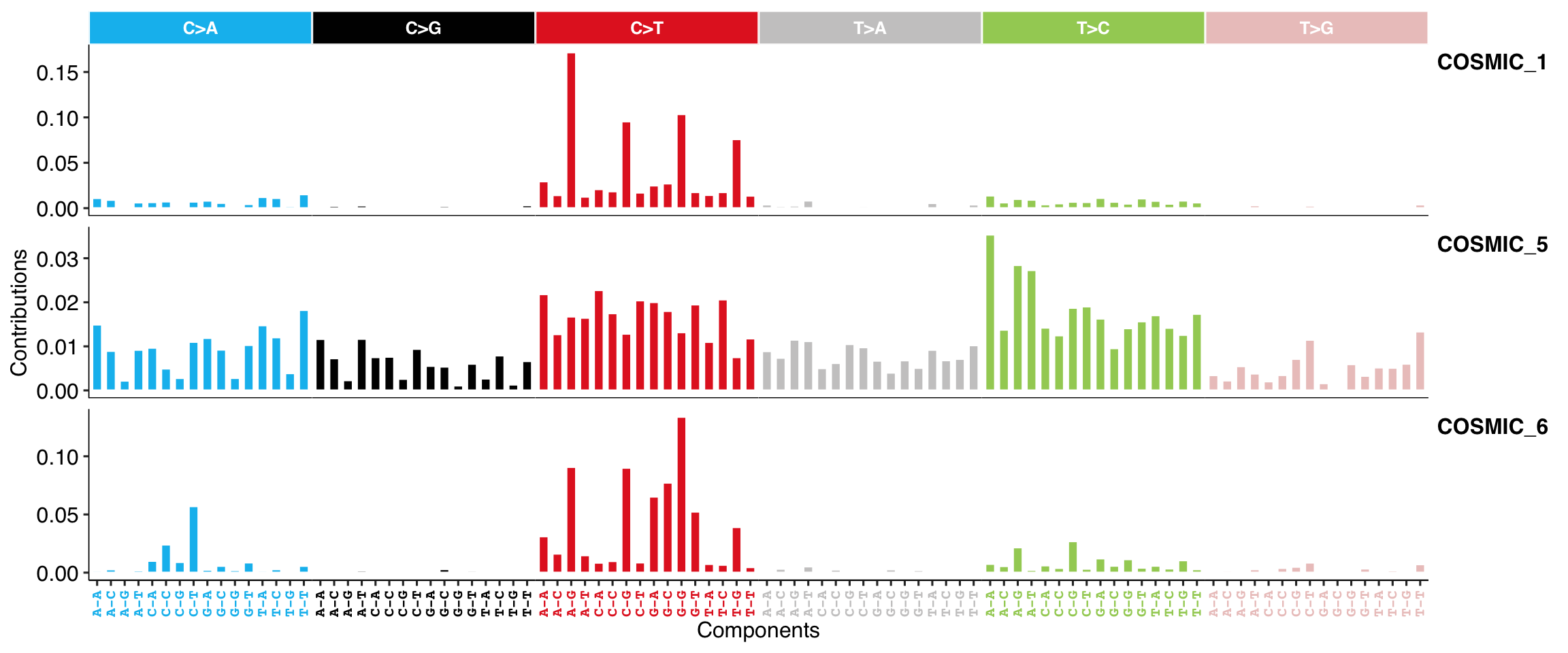
show_cosmic_sig_profile(sig_index = c(1, 2, 3), style = "cosmic", sig_db = "DBS")
#>
#> Valid index for db 'DBS':
#> 1 2 3 4 5 6 7 8 9 10 11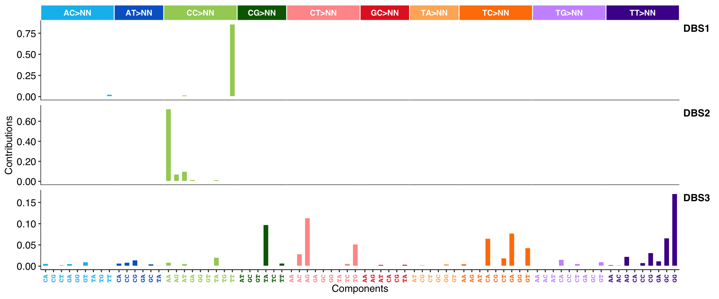
show_cosmic_sig_profile(sig_index = c(4, 5, 6), style = "cosmic", sig_db = "ID")
#>
#> Valid index for db 'ID':
#> 1 2 3 4 5 6 7 8 9 10 11 12 13 14 15 16 17 18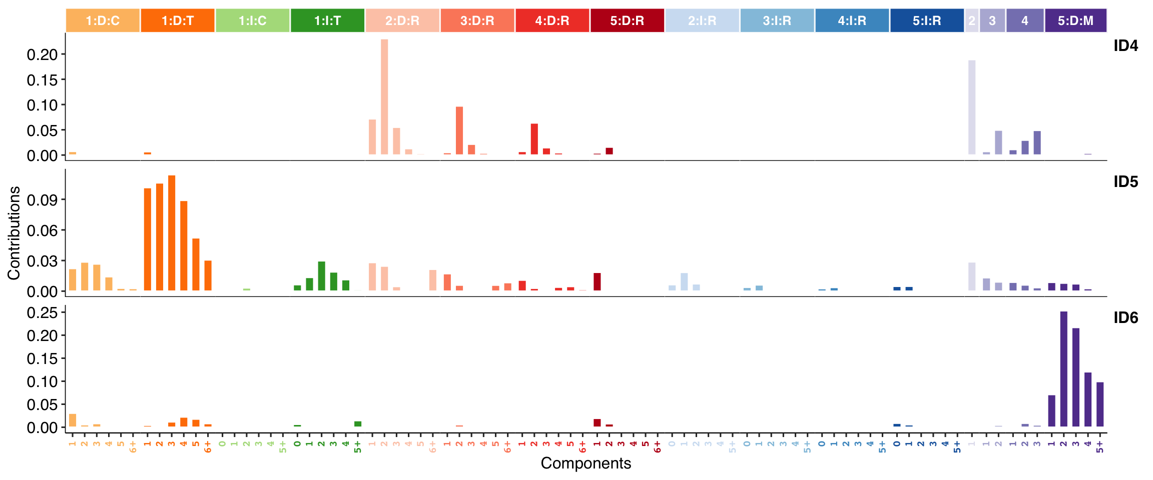
8.2 Exposure Profile
show_sig_exposure(mt_sig)
show_sig_exposure(mt_sig, style = "cosmic")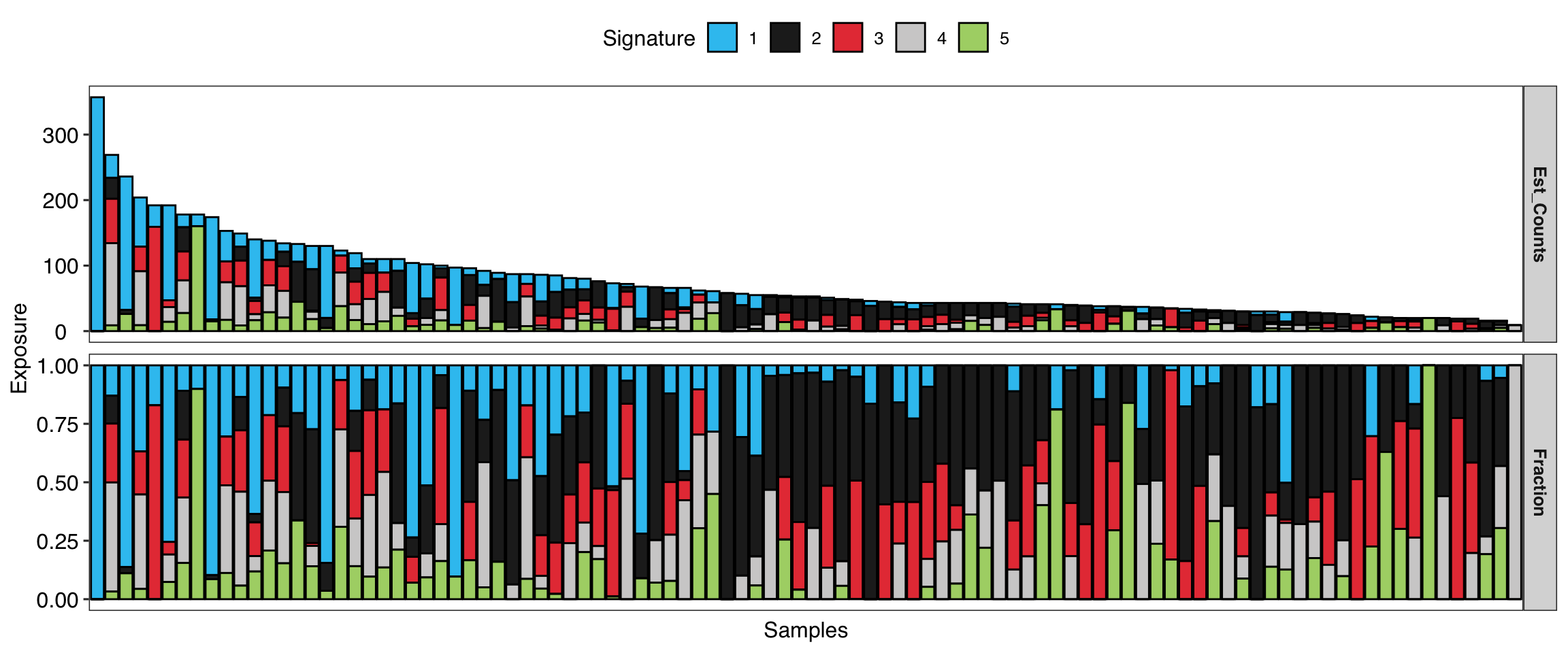
show_sig_exposure(sig_w, style = "cosmic")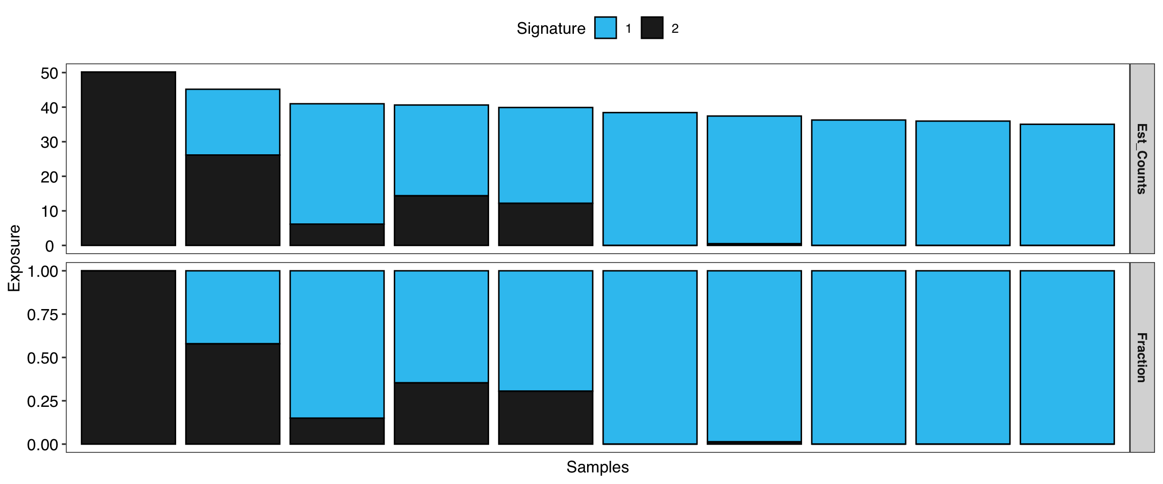
You can put group labels in the exposure profile.
grp <- get_groups(sig_w)
#> ℹ [2021-05-18 23:17:24]: Started.
#> ✓ [2021-05-18 23:17:24]: 'Signature' object detected.
#> ℹ [2021-05-18 23:17:24]: Obtaining clusters from the hierarchical clustering of the consensus matrix...
#> ℹ [2021-05-18 23:17:24]: Finding the dominant signature of each group...
#> => Generating a table of group and dominant signature:
#>
#>     Sig1 Sig2
#>   1    0    2
#>   2    8    0
#> => Assigning a group to a signature with the maxium fraction (stored in 'map_table' attr)...
#> ℹ [2021-05-18 23:17:24]: Summarizing...
#>  group #1: 2 samples with Sig2 enriched.
#>  group #2: 8 samples with Sig1 enriched.
#> ! [2021-05-18 23:17:24]: The 'enrich_sig' column is set to dominant signature in one group, please check and make it consistent with biological meaning (correct it by hand if necessary).
#> ℹ [2021-05-18 23:17:24]: 0.066 secs elapsed.
grp_label <- grp$group
names(grp_label) <- grp$sampleshow_sig_exposure(sig_w, style = "cosmic", groups = grp_label)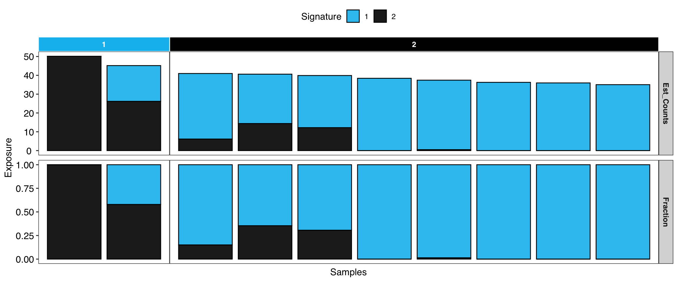
Of note:
- For COSMIC signatures, the absolute exposure is the estimated mutation counts.
- For copy number signatures, the absolute exposure is the estimated copy number segments.
8.3 Consensus Map
This can only support the result from sig_extract() with multiple runs.
show_sig_consensusmap(mt_sig)
8.4 Catalogue Profile
Based on plot method for signature, we can plot raw catalogue profile.
show_catalogue(t(mt_tally$nmf_matrix), style = "cosmic", x_label_angle = 90)
At default, the function sums all samples. Users can specify sample ID.
show_catalogue(t(mt_tally$nmf_matrix), style = "cosmic", samples = "TCGA-E9-A22E-01A-11D-A159-09", x_label_angle = 90)